Iterative Methods for the Computation of the Perron Vector of Adjacency Matrices ^†

Abstract

The power method is commonly applied to compute the Perron vector of large adjacency matrices. Blondel et al. [SIAM Rev. 46, 2004] investigated its performance when the adjacency matrix has multiple eigenvalues of the same magnitude. It is well known that the Lanczos method typically requires fewer iterations than the power method to determine eigenvectors with the desired accuracy. However, the Lanczos method demands more computer storage, which may make it impractical to apply to very large problems. The present paper adapts the analysis by Blondel et al. to the Lanczos and restarted Lanczos methods. The restarted methods are found to yield fast convergence and to require less computer storage than the Lanczos method. Computed examples illustrate the theory presented. Applications of the Arnoldi method are also discussed.

1. Introduction

Networks arise in many areas, such as social media, transportation, and chemistry; see [1,2] for many examples. Networks can be represented by graphs $\mathcal{G}$ that are made up of a set of vertices or nodes $\mathcal{V}={\left\{v_i\right\}}_{i=1}^n$ and a set of edges $\mathcal{E}={\left\{e_i\right\}}_{i=1}^m$, connecting the nodes. Two distinct nodes, $v_i$ and $v_j$, are said to be adjacent if there is an edge between them. The analysis of graphs by mathematical and computational methods can provide valuable information about the networks they model and is receiving considerable attention.

This paper considers networks that can be represented by simple unweighted graphs, that is, no edge starts and ends at the same node, and there is at most one edge between each pair of distinct nodes. Extension to weighted simple graphs, in which each edge has a positive weight, is straightforward. A graph is said to be undirected if every edge is a “two-way street”; a graph with at least one edge that is a “one-way street” is said to be directed. A directed edge $e_k$ pointing from vertex $v_i$ to vertex $v_j$ can be identified with the ordered pair $(v_i,v_j)$; for an undirected edge, this pair is not ordered. A walk of length k in a graph is a sequence of $k+1$ vertices $v_{i_1},v_{i_2},\dots ,v_{i_{k+1}}$ and a sequence of k edges $e_{j_1},e_{j_2},\dots ,e_{j_k}$, not necessarily distinct, such that $e_{j_p}$ points from $v_{i_p}$ to $v_{i_{p+1}}$ in a directed graph, or connects $v_{i_p}$ to $v_{i_{p+1}}$ in an undirected graph, for $p=1,2,\dots ,k$. A path is a walk in which all the nodes are distinct.

An unweighted simple graph $\mathcal{G}$ with n nodes can be represented by its adjacency matrix $A={\left[a_{ij}\right]}_{i,j=1}^n\in {\mathbb{R}}^{n\times n}$, where $a_{ij}=1$ when there is an edge from vertex $v_i$ to vertex $v_j$; otherwise, $a_{ij}=0$. In particular, $a_{ii}=0$ for all i. Undirected graphs are associated with symmetric adjacency matrices, while the adjacency matrix for a directed graph is non-symmetric. Typically, the number of edges, m, is much smaller than $n^2$. This makes the adjacency matrix A sparse. An undirected graph is said to be connected if there is a path connecting each pair of nodes. A directed graph is referred to as strongly connected if there is a directed path from $v_i$ to $v_j$ and vice versa for every pair of distinct nodes. The adjacency matrix A associated with an undirected graph $\mathcal{G}$ is irreducible if and only if $\mathcal{G}$ is connected. Similarly, the adjacency matrix A associated with a directed graph $\mathcal{G}$ is irreducible if and only if $\mathcal{G}$ is strongly connected.

A problem of considerable interest in network analysis is the determination of the most important vertices of a network. The notion of centrality can be used to identify these vertices. There are many centrality measures available, including degree centrality [1,2], betweenness centrality [3], hub-and-authority centrality [4], and eigenvector centrality [5].

We are interested in investigating the performance of iterative methods for determining the eigenvector centrality of vertices belonging to certain structured graphs $\mathcal{G}$ with many nodes n. The eigenvector centrality was introduced by Bonacich for quantifying the influence a node has in a network [5], beyond its nearest neighbors, in terms of spectral properties of the associated adjacency matrix. According to the Perron–Frobenius theorem, the largest eigenvalue, $\rho$, which is known as the Perron root, of a nonnegative irreducible matrix A, is unique and has a unique eigenvector $\mathbf{w}={[w_1,w_2,\dots ,w_n]}^T\in {\mathbb{R}}^n$ (up to scaling) with positive components $w_i$. This vector is commonly referred to as the Perron vector of A; see, for example, Meyer ([6] Section 8.3). For notational simplicity, we may assume that $\mathbf{w}$ is scaled so that $\parallel \mathbf{w}\parallel =1$. Here and throughout this paper, $\parallel ·\parallel$ denotes the Euclidean vector norm. The eigenvector centrality of the vertex $v_i$ is given by the entry $w_i$ of the Perron vector $\mathbf{w}$ of the adjacency matrix A. A vertex $v_i$ is considered a central, that is, important, vertex of the graph $\mathcal{G}$ if $w_i$ is the largest entry of $\mathbf{w}$. This centrality measure also takes into account the centralities of those nodes to which $v_i$ is connected [7].

Blondel et al. [8] investigated the performance of the power method when applied to determining the Perron vector of a matrix of the form

$$M=\left[\begin{array}{cc}0& A\\ A^T& 0\end{array}\right]\in {\mathbb{R}}^{2n\times 2n},$$

(1)

where $A\in {\mathbb{R}}^{n\times n}$ is the adjacency matrix for a graph $\mathcal{G}$ with n nodes, and the superscript T denotes transposition. M can be interpreted as the adjacency matrix of a bipartite graph containing $2n$ vertices partitioned into two disjoint vertex subsets, whose connections are described by A and occur only across, but not within, the two groups.

There are numerous methods for partitioning the vertex set of a bipartite graph $\mathcal{G}$ so that its adjacency matrix is of the form (1); see [2,9,10] and references therein. The Perron vector of the matrix (1) is used to determine the hub-and-authority centralities for the vertices of $\mathcal{G}$ [2,4] and its components give similarity scores between graph nodes. These scores were introduced by Blondel et al. [8]. There are several applications of similarity scores. These applications lead to the construction of a self-similarity matrix associated with a graph, which measures how vertices are similar to each other [8]; see [11] for an application in archaeology of the similarity matrix associated with a bipartite graph and for an algorithm for solving the seriation problem. The latter is a fundamental ordering problem that aims at finding the best enumeration order of a set of units so that in the resulting sequence, elements having higher similarity are placed close to each other.

Given an initial vector ${\mathbf{z}}_0\in {\mathbb{R}}^{2n}$ with positive entries, the power method applied to the matrix M generates the sequence of vectors

$${\mathbf{z}}_k=\frac{M{\mathbf{z}}_{k-1}}{{\parallel M{\mathbf{z}}_{k-1}\parallel }_2},k=1,2,\dots .$$

(2)

When applied to a real square matrix with a single largest eigenvalue of maximal magnitude, the power method is known to determine a sequence of vectors that converge to the span of the eigenvector associated with this eigenvalue for almost all initial vectors; see, for example, Saad ([12] Section 4.1). The following result, which highlights the property of the adjacency matrix of a bipartite graph of having a spectrum symmetric with respect to the origin ([13] Theorem 3.14), shows why the application of the power method to the matrix (1) is not straightforward.

Proposition 1.

The matrix (1) has distinct eigenvalues of the largest magnitude.

Proof. 

Partition the Perron vector $\mathbf{x}={[{\mathbf{x}}_1^T,{\mathbf{x}}_2^T]}^T\in {\mathbb{R}}^{2n}$ of the matrix M defined by (1), where ${\mathbf{x}}_i\in {\mathbb{R}}^n$, $i=1,2$. Let $\lambda$ denote the Perron root of M. Then, $M\mathbf{x}=\lambda \mathbf{x}$ implies that

$$M\left[\begin{array}{c}{\mathbf{x}}_1\\ -{\mathbf{x}}_2\end{array}\right]=-\lambda \left[\begin{array}{c}{\mathbf{x}}_1\\ -{\mathbf{x}}_2\end{array}\right].$$

Thus, the negative Perron root is also an eigenvalue of M. □

The presence of more than one eigenvalue of the largest magnitude of M suggests that the sequence of vectors, ${\mathbf{z}}_1,{\mathbf{z}}_2,{\mathbf{z}}_3,\dots$, might not converge to the Perron vector. Indeed, Blondel et al. [8] show that both the limits

$$\underset{k\to \infty }{lim}{\mathbf{z}}_{2k}\mathrm{and}\underset{k\to \infty }{lim}{\mathbf{z}}_{2k-1}$$

(3)

exist, but they might not be the same. The limits depend on the initial vector ${\mathbf{z}}_0$ for the power iteration and none of the limits might be the Perron vector for M. Throughout this paper, $\mathbf{e}={[1,1,\dots ,1]}^T$ denotes the vector with all entries 1 of a suitable dimension. Blondel at al. ([8] Theorem 2) show that when ${\mathbf{z}}_0=\mathbf{e}/\parallel \mathbf{e}\parallel$, the limit on the left-hand side of (3) is the Perron vector for M.

An advantage of the power method, when compared to other methods for computing the Perron vector of a matrix with only nonnegative entries, is that only two vectors, ${\mathbf{z}}_k$ and $M{\mathbf{z}}_k$, have to be stored simultaneously during the computations. The low storage requirement may be important for very large matrices; however, convergence of the power method can also be very slow when there is only one eigenvalue of the largest magnitude. The rate of convergence decreases with the distance between the Perron root and the magnitude of the second largest eigenvalue in modulus; see, for example, ([12] Section 4.1). It is therefore interesting to investigate the convergence properties of methods that converge faster, such as the Lanczos or restarted Lanczos methods, when applied to matrices of the form (1) and generalizations thereof. It is the purpose of the present paper to study the convergence of the Lanczos and restarted Lanczos methods when applied to the computation of the Perron vector of matrices of the form (1) and some generalizations. Our analysis is based on results by Blondel et al. [8]. We also discuss the computation of the Perron vector of structured matrices, somewhat related to the matrix M, and by application of the Arnoldi method to the submatrix A in (1). These particular matrices represent graphs with a chained structure that refine the notion of bipartivity [14].

This paper is organized as follows: Section 2 introduces undirected chained graphs. The adjacency matrix for this kind of graph has a staircase structure, which generalizes the structure (1). Chained graphs have been shown to be bipartite in [14], which implies that the eigenvalues of their associated adjacency matrices appear in ± pairs. Section 3 studies the performance of the Lanczos and restarted Lanczos methods when applied to computing the Perron vector for these and other symmetric adjacency matrices. The Arnoldi method and its application to estimating the Perron vector for a symmetric matrix considered by Blondel et al. [8] are described in Section 4. A few computed examples are presented in Section 5, and Section 6 contains concluding remarks.

2. Undirected Chained Graphs

This section describes ℓ-chained undirected graphs and the structure of their adjacency matrices. These graphs, which are particular bipartite graphs, were introduced in [14] and are defined as follows.

Definition 1.

An undirected graph $\mathcal{G}=\{\mathcal{V},\mathcal{E}\}$ is said to be ${\ell }_i$-chainedwith initial vertex $v_i$ if the set of vertices can be subdivided into ${\ell }_i$ disjoint non-empty subsets

$$\mathcal{V}={\mathcal{V}}_1\cup {\mathcal{V}}_2\cup \cdots \cup {\mathcal{V}}_{{\ell }_i},$$

such that $v_i\in {\mathcal{V}}_1$, and all vertices in the set ${\mathcal{V}}_j$, are adjacent only to vertices in the sets ${\mathcal{V}}_{j-1}$ or ${\mathcal{V}}_{j+1}$ for $j=2,3,\dots ,{\ell }_i-1$, where the chain length ${\ell }_i$ is the largest number of vertex subsets ${\mathcal{V}}_j$ with this property. Moreover, the vertices in ${\mathcal{V}}_1$ and ${\mathcal{V}}_{{\ell }_i}$ are adjacent only to vertices in ${\mathcal{V}}_2$ and ${\mathcal{V}}_{{\ell }_i-1}$, respectively. Vertex sets ${\mathcal{V}}_j$ with consecutive indices are said to be adjacent.

Chained graphs arise in various applications; see [8,14,15] and Section 5.

Consider an undirected ℓ-chained graph $\mathcal{G}=(\mathcal{V},\mathcal{E})$ with vertex set partitioning $\mathcal{V}={\mathcal{V}}_1\cup {\mathcal{V}}_2\cup \cdots \cup {\mathcal{V}}_{\ell }$. Let $n_i$ be the cardinality of the vertex subset ${\mathcal{V}}_i$ for $i=1,2,\cdots ,\ell$. Thus, the graph $\mathcal{G}$ has $n={\sum }_{i=1}^{\ell }{n}_i$ nodes. Order the vertices $v_j$ of $\mathcal{G}$ so that the vertices in ${\mathcal{V}}_i$ precede those in ${\mathcal{V}}_{i+1}$ for $i=1,2,\dots ,\ell -1$, and define the matrix $A_i\in {\mathbb{R}}^{n_i\times n_{i+1}}$ that describes the connections between the vertices in ${\mathcal{V}}_i$ and the vertices in ${\mathcal{V}}_{i+1}$ for $i=1,2,\cdots ,\ell -1$. Then, the adjacency matrix $M\in {\mathbb{R}}^{n\times n}$, associated with $\mathcal{G}$, has the staircase structure

$$M=\left[\begin{array}{cc}O& A_1\\ A_1^T& O& A_2\\ & A_2^T& \ddots & \ddots \\ & & \ddots & O& A_{\ell -1}\\ & & & A_{\ell -1}^T& O\end{array}\right].$$

(4)

Theorem 1

([14]). An ℓ-chained graph is bipartite. Conversely, if a graph is bipartite, then the graph is ℓ-chained for some $\ell \ge 2$.

From Theorem 1 it follows that, for a suitable permutation matrix $P\in {\mathbb{R}}^{n\times n}$, the adjacency matrix (4) can be permuted to the form

$$PM{P}^T=\left[\begin{array}{cc}O& C\\ C^{T\phantom{{}^1}}& O\end{array}\right],$$

(5)

with $C\in {\mathbb{R}}^{n_o\times n_e}$, where

$$n_o=\sum _{i=1}^{\lfloor (\ell +1)/2\rfloor }{n}_{2i-1},n_e=\sum _{i=1}^{\lfloor \ell /2\rfloor }{n}_{2i}.$$

Here, $\lfloor \alpha \rfloor$ denotes the integer part of $\alpha \ge 0$. The structure (5) is the same as (1). It follows from Proposition 1 that the adjacency matrix for an ℓ-chained undirected graph has pairs of eigenvalues of the opposite sign, which include the Perron root.

Example 1.

Consider the 3-chained graph with adjacency matrix

$$M=\left[\begin{array}{ccc}O& A& O\\ A^T& O& A\\ O& A^T& O\end{array}\right]\in {\mathbb{R}}^{3n\times 3n},$$

(6)

where $A\in {\mathbb{R}}^{n\times n}$. Then

$$M^2=\left[\begin{array}{ccc}A{A}^T& O& AA\\ O& A^{T}A+A{A}^T& O\\ A^T{A}^T& O& A^{T}A\end{array}\right].$$

(7)

Introduce the permutation matrix

$$P=\left[\begin{array}{ccc}{I}_n& O& O\\ O& O& I_n\\ O& I_n& O\end{array}\right],$$

where $I_n\in {\mathbb{R}}^{n\times n}$ is the identity matrix. Then, the matrix $C\in {\mathbb{R}}^{2n\times n}$ is defined by

$$PM{P}^T=\left[\begin{array}{ccc}O& O& A\\ O& O& A^T\\ A^T& A& O\end{array}\right]=\left[\begin{array}{cc}O& C\\ C^{T\phantom{{}^1}}& O\end{array}\right].$$

It follows that the ± singular values of C are eigenvalues of M. This yields $2n$ of the eigenvalues of M. The remaining n eigenvalues vanish. We will discuss the computation of the Perron vector of matrices of the form (6), as well as of matrices of the form (4), in the following section.

3. The Lanczos and Restarted Lanczos Methods

This section discusses the application of the Lanczos and restarted Lanczos methods to the computation of the Perron vector of an undirected connected graph. We first consider the Lanczos method and subsequently turn to restarted variants.

The Lanczos method reduces a large symmetric matrix to a usually much smaller symmetric tridiagonal matrix by computing an orthogonal projection onto a Krylov subspace of fairly low dimension. It is a commonly used method for determining approximations of a few large eigenvalues and associated eigenvectors of a large symmetric matrix; see, for example, [12] for a discussion of this method.

Consider an undirected connected graph $\mathcal{G}$ with associated adjacency matrix $A\in {\mathbb{R}}^{n\times n}$. Application of $1\le k\ll n$ steps of the Lanczos method to A with initial vector $\mathbf{v}\in {\mathbb{R}}^n\backslash \left\{\mathbf{0}\right\}$ yields, generically, the Lanczos decomposition

$$A{Q}_k=Q_k{T}_k+{\beta }_k{\mathbf{q}}_{k+1}{\mathbf{e}}_k^T,$$

(8)

where the columns of the matrix $Q_k=[{\mathbf{q}}_1,{\mathbf{q}}_2,\dots ,{\mathbf{q}}_k]\in {\mathbb{R}}^{n\times k}$ form an orthonormal basis for the Krylov subspace,

$${\mathcal{K}}_k(A,\mathbf{v})=span\{\mathbf{v},A\mathbf{v},A^2\mathbf{v},\dots ,A^{k-1}\mathbf{v}\},k=1,2,\dots ,$$

with ${\mathbf{q}}_1=\mathbf{v}/\parallel \mathbf{v}\parallel$. Throughout this paper, ${\mathbf{e}}_k={[0,\dots ,0,1,0,\dots ,0]}^T$ denotes the kth axis vector of the suitable dimension. Moreover,

$$T_k=\left[\begin{array}{ccccc}{\alpha }_1& {\beta }_1& & & \\ {\beta }_1& {\alpha }_2& {\beta }_2& & \\ & \ddots & \ddots & \ddots & \\ & & {\beta }_{k-2}& {\alpha }_{k-1}& {\beta }_{k-1}\\ & & & {\beta }_{k-1}& {\alpha }_k\end{array}\right]\in {\mathbb{R}}^{k\times k}$$

is a symmetric tridiagonal matrix, the coefficient ${\beta }_k$ in (8) is positive, and the vector ${\mathbf{q}}_{k+1}\in {\mathbb{R}}^n$ satisfies $Q_k^T{\mathbf{q}}_{k+1}=\mathbf{0}$ and $\parallel {\mathbf{q}}_{k+1}\parallel =1$. We tacitly assume that the number of steps k of the Lanczos method is small enough so that the decomposition (8) with the stated properties exists. This is the generic situation.

Let ${\rho }_k$ denote the largest eigenvalue of $T_k$, and let ${\mathbf{y}}_k\in {\mathbb{R}}^k$ be an associated unit eigenvector. Then, ${\rho }_k$ and $Q_k{\mathbf{y}}_k$ are commonly referred to as a Ritz value and a Ritz vector, respectively, of A.

Theorem 2.

Consider an undirected connected graph $\mathcal{G}$ with adjacency matrix $M\in {\mathbb{R}}^{n\times n}$. Then, M is symmetric and nonnegative. Let ρ denote the Perron root of M and let $\mathbf{w}$ be the associated Perron vector. Apply k steps of the Lanczos method to M with initial vector $\mathbf{e}={[1,1,\dots ,1]}^T\in {\mathbb{R}}^n$. This produces the decompositions

$$M{Q}_k=Q_k{T}_k+{\beta }_k{\mathbf{q}}_{k+1}{\mathbf{e}}_k^T,k=0,1,\dots .$$

(9)

Let ${\rho }_k$ denote the largest eigenvalue of $T_k$ with the associated Perron vector ${\mathbf{y}}_k$. Then, the Ritz values ${\rho }_k$ converge to the Perron root ρ of M and the Ritz vectors ${\mathbf{w}}_k=Q_k{\mathbf{y}}_k$ converge to $\mathbf{w}$ as k increases. If the Lanczos method breaks down at iteration ℓ, then ${\mathbf{w}}_{\ell }$ is the Perron vector.

Proof. 

The eigenvectors of M are stationary points of the Rayleigh quotient

$$r(\mathbf{x})=\frac{{\mathbf{x}}^{T}M\mathbf{x}}{{\mathbf{x}}^T\mathbf{x}},\mathbf{x}\in {\mathbb{R}}^n\backslash \left\{\mathbf{0}\right\},$$

and the eigenvalues of M are the values of $r(\mathbf{x})$ at these stationary points. The Perron root $\rho$ is the maximum value of $r(\mathbf{x})$. The largest eigenvalue of $T_k$ is the maximum value ${\rho }_k$ of $r(\mathbf{x})$ over the k-dimensional Krylov subspace ${\mathcal{K}}_k(M,\mathbf{e})$. It follows that ${\rho }_k\le \rho$.

Blondel et al. ([8] Theorem 2) show that, using the initial vector $\mathbf{e}/\parallel \mathbf{e}\parallel$, the sequence ${\mathbf{z}}_{2k}$ in (2) generated by the power method converges to the Perron vector $\mathbf{w}$ of M. The unit vector ${\mathbf{z}}_{2k}$ lives in ${\mathcal{K}}_{2k}(M,\mathbf{e})$. Clearly,

$${\mathbf{z}}_{2k}^{T}M{\mathbf{z}}_{2k}\le {\rho }_{2k}\le \rho .$$

(10)

Since the Krylov subspaces ${\mathcal{K}}_j(M,\mathbf{e})$, $j=1,2,\dots$ are nested, it follows that

$${\rho }_{2k-2}\le {\rho }_{2k-1}\le {\rho }_{2k}.$$

(11)

It is a consequence of the mentioned result by Blondel et al. [8] that the Lanczos method does not break down until the Perron vector has been determined. Assume, to the contrary, that the Lanczos method breaks down at step k. Then, the relation (9) is replaced by

$$M{Q}_k=Q_k{T}_k,$$

which shows that the range of $Q_k$ forms an invariant subspace of M. This implies that the vector $M{\mathbf{z}}_k$, determined by the power method in the next step, lives in the range of $Q_k$. This would imply that the Perron root of M is the Perron root of $T_k$, and therefore the Lanczos method determines the Perron root and Perron vector.

It follows from (10) that ${\rho }_{2k}$ converges to $\rho$ and, due to (11), the sequence ${\rho }_j$ converges monotonically to $\rho$ (from below) as j increases. Let ${\mathbf{y}}_j\in {\mathbb{R}}^j$ be the Perron vector of $T_j$. Since $T_j$ is an irreducible symmetric tridiagonal matrix, the unit vector ${\mathbf{y}}_j$ is uniquely determined. Then, the associated Ritz vectors ${\mathbf{w}}_j=Q_j{\mathbf{y}}_j$ converge to the Perron vector of M as j increases. We remark that the Ritz vectors ${\mathbf{w}}_j$ so obtained, $j\ge 1$, may have small negative entries. This is of no importance, since we are interested in determining the largest component(s) of these vectors. □

The iterations of the Lanczos method applied to M are terminated as soon as two consecutive approximations ${\mathbf{w}}_{k-1}$ and ${\mathbf{w}}_k$ of the Perron vector are close enough, that is, as soon as

$$\parallel {\mathbf{w}}_k-{\mathbf{w}}_{k-1}\parallel \le ϵ,$$

(12)

for some user-specified (small) value of $ϵ>0$. Note that

$$\parallel {\mathbf{w}}_k-{\mathbf{w}}_{k-1}\parallel =\parallel Q_k{\mathbf{y}}_k-Q_{k-1}{\mathbf{y}}_{k-1}\parallel =∥{\mathbf{y}}_k-\left[\begin{array}{c}{\mathbf{y}}_{k-1}\\ 0\end{array}\right]∥.$$

Thus, it suffices to choose a k large enough so that

$$∥{\mathbf{y}}_k-\left[\begin{array}{c}{\mathbf{y}}_{k-1}\\ 0\end{array}\right]∥\le ϵ.$$

The Lanczos iteration is described by Algorithm 1. The algorithm applies the Lanczos method to a general real symmetric matrix $M\in {\mathbb{R}}^{n\times n}$. In Line 14 of the algorithm, the symmetric tridiagonal matrix $T_{k-1}\in {\mathbb{R}}^{(k-1)\times (k-1)}$ is augmented by appending a row and a column to obtain the new symmetric tridiagonal matrix $T_k\in {\mathbb{R}}^{k\times k}$.

Algorithm 1 Determine the Perron vector of the matrix M by the Lanczos method.

Require:  Adjacency matrix $M\in {\mathbb{R}}^{n\times n}$ and initial vector $\mathbf{e}=\mathbf{1}$. Ensure:  Approximation $\mathbf{w}$ of the Perron vector of M.  1: ${\beta }_0=0$, ${\mathbf{q}}_0=\mathbf{0}$, ${\mathbf{q}}_1=\frac{\mathbf{e}}{∥\mathbf{e}∥}$, ${\mathbf{w}}_0=\mathbf{0}$, $k=1$  2: ${\alpha }_1={\mathbf{q}}_1^{T}M{\mathbf{q}}_1$  3: $\mathbf{r}=M{\mathbf{q}}_1-{\alpha }_1{\mathbf{q}}_1$  4: ${\beta }_1=∥\mathbf{r}∥$  5: ${\mathbf{q}}_2=\mathbf{r}/{\beta }_1$  6: $T_1={\alpha }_1$  7: $Q_1={\mathbf{q}}_1$, ${\mathbf{w}}_1={\mathbf{q}}_1$  8: while$∥{\mathbf{w}}_k-{\mathbf{w}}_{k-1}∥>ϵ$do  9:   $k=k+1$ 10:   ${\alpha }_k={\mathbf{q}}_k^{T}M{\mathbf{q}}_k$ 11:   $\mathbf{r}=M{\mathbf{q}}_k-{\alpha }_k{\mathbf{q}}_k-{\beta }_{k-1}{\mathbf{q}}_{k-1}$ 12:   ${\beta }_k=∥\mathbf{r}∥$ 13:   ${\mathbf{q}}_{k+1}=\mathbf{r}/{\beta }_k$ 14:   $T_k=\left[\begin{array}{cc}{T}_{k-1}& {\beta }_{k-1}{\mathbf{e}}_{k-1}\\ {\beta }_{k-1}{\mathbf{e}}_{k-1}^T& {\alpha }_k\end{array}\right]$ 15:   $Q_k=\left[Q_{k-1}{\mathbf{q}}_k\right]$ 16:  Compute the Perron vector ${\mathbf{y}}_k$ of $T_k$ 17:   ${\mathbf{w}}_k=Q_k{\mathbf{y}}_k$ 18: end while 19: $\mathbf{w}={\mathbf{w}}_k$

The following example compares the results of finding the most important vertices of each vertex subset of an undirected 4-chained graph by the power method and the Lanczos method with initial vector $\mathbf{e}$. In this comparison, we terminate the iterations with the power method as soon as two consecutive approximations ${\mathbf{z}}_{2k}$ and ${\mathbf{z}}_{2(k-1)}$ of the Perron vector are sufficiently close, that is, as soon as

$$\parallel {\mathbf{z}}_{2k}-{\mathbf{z}}_{2(k-1)}\parallel \le ϵ.$$

(13)

Example 2.

This example uses the Citeseer Index data set downloaded on June 2007 from the $Citesee{r}^X$ website [16]. The data set consists of a list of papers with some information such as authors, journals, and institutions. We extracted an undirected 4-chained network from this data set. It shows relations between the vertex subsets institutions, authors, papers and journals. The number of vertices that represent institutions, authors, papers and journals are 20, 58, 26 and 21, respectively. The power method and the Lanczos method are applied with the stopping criteria (13) and (12), respectively, with $ϵ={10}^{-4}$.

Both the power and Lanczos methods identify vertex $v_1$ as the most important university, vertices $v_{21}$ and $v_{22}$ as the most important authors, vertex $v_{81}$ as the most important paper, and vertex $v_{108}$ as the most important journal. The power method terminates the iterations after step 364, while the Lanczos method stops at step 26. Thus, the Lanczos method requires the evaluation of significantly fewer matrix–vector products with the matrix M than the power method to determine the most important vertices of each vertex subset.

Typically, the Lanczos method yields much faster convergence to the Perron vector of a symmetric nonnegative matrix M than the power method. However, it has the drawback of requiring storage space for the matrix $Q_k$ in (9). The need to store the matrix $Q_k$ may make it difficult to apply the Lanczos method to compute the Perron vector of very large adjacency matrices. We describe two standard approaches for circumventing this difficulty. They restart the Lanczos iterations in different ways.

(i)

Carry out the Lanczos iterations twice: First generate the tridiagonal matrix $T_k$ for a suitably chosen k (see below) and discard the columns of the matrix $Q_k$ that are not required by the Lanczos method for determining the next column. Indeed, to compute column ${\mathbf{q}}_{j+1}$ for $j\ge 2$ only the columns ${\mathbf{q}}_j$ and ${\mathbf{q}}_{j-1}$ are needed. Thus, the storage demand is modest and bounded independently of the number of Lanczos steps k. Having computed the Perron vector ${\mathbf{y}}_k$ for $T_k$, we have to evaluate the corresponding Ritz vector ${\mathbf{w}}_k=Q_k{\mathbf{y}}_k$. This can be done by regenerating the columns of $Q_k$. Thus, we determine these columns by applying the recursion formula of the Lanczos method again and discard the columns ${\mathbf{q}}_j$ as soon as their contribution to the Ritz vector ${\mathbf{w}}_k$ have been evaluated. The inner products that determine the nontrivial entries of $T_k$ do not have to be recomputed. This approach of reducing the storage amount is straightforward, but it doubles the number of matrix–vector product evaluations with M. This method is described by Algorithm 2. The iterations are terminated similarly as in Algorithm 1.

(ii)

Restart the Lanczos method, that is, compute an approximation of the Perron vector every k iteration, and use this approximation as a new initial vector when restarting the Lanczos iterations. The vector $\mathbf{e}$ is used to initialize the very first k Lanczos steps. The method is restarted until the stopping criterion is satisfied. The storage requirement of this restarted Lanczos method is limited to essentially the matrix $Q_k$, independently of the number of iterations that are carried out. However, the rate of convergence of computed approximations of the Perron vector may be slower than for the un-restarted Lanczos method. This method is discussed in Theorem 3 below.

Example 3.

We applied Algorithm 2 to the adjacency matrix of the 4-chained network described in Example 2, with $ϵ={10}^{-4}$. The stopping criterion was satisfied at step 20. The algorithm determined the same vertices as the standard Lanczos method in Example 2. The main differences between Algorithm 1 and Algorithm 2 are that the latter requires less computer storage, but more matrix–vector product evaluations with M (40 vs. 26). The difference in the number of steps required by Algorithms 1 and 2 depends in part on the different stopping criteria used. In Algorithm 1, the iterations are terminated when two consecutive Ritz vectors are close enough, while Algorithm 2 is terminated when two consecutive Ritz values are sufficiently close.

We turn to computing the Perron vector of M by the restarted Lanczos method described in (ii). This method applies k steps of the Lanczos method to the matrix M with initial vector $\mathbf{e}$ to determine the decomposition (9), and computes the Perron vector ${\mathbf{y}}^{(1)}\in {\mathbb{R}}^k$ of the symmetric tridiagonal matrix $T_k$ in this decomposition. We denote the Perron root of $T_k$ by ${\rho }^{(1)}$. Then, $Q_k{\mathbf{y}}^{(1)}$ is the Ritz vector of M that best approximates the Perron vector, and ${\rho }^{(1)}$ is the corresponding Ritz value. The computed Ritz vector may have negative entries, while the Perron vector of M is known to only have strictly positive entries. We therefore set all entries of $Q_k{\mathbf{y}}^{(1)}$ that are smaller than a small $\delta >0$, say $\delta ={10}^{-8}$, to $\delta$, and refer to the vector so obtained as ${\widehat{\mathbf{z}}}^{(1)}$.

Algorithm 2 Determine the Perron vector of the matrix M by applying twice the Lanczos recursions.

Require:  Adjacency matrix $M\in {\mathbb{R}}^{n\times n}$ and initial vector $\mathbf{e}=\mathbf{1}$. Ensure:  Approximation $\mathbf{w}$ of the Perron vector of M.  1: ${\beta }_0=0$, ${\mathbf{q}}_1=\mathbf{e}/\parallel \mathbf{e}\parallel$, ${\rho }_0=0$, $k=1$  2: ${\alpha }_1={\mathbf{q}}_1^{T}M{\mathbf{q}}_1$  3: $\mathbf{r}=M{\mathbf{q}}_1-{\alpha }_1{\mathbf{q}}_1$  4: ${\beta }_1=∥\mathbf{r}∥$  5: ${\mathbf{q}}_0={\mathbf{q}}_1$  6: ${\mathbf{q}}_1=\mathbf{r}/{\beta }_1$  7: $T_1={\alpha }_1$, ${\rho }_1={\alpha }_1$  8: while$|{\rho }_k-{\rho }_{k-1}|>ϵ$do  9:   $k=k+1$ 10:   ${\alpha }_k={\mathbf{q}}_1^{T}M{\mathbf{q}}_1$ 11:   $\mathbf{r}=M{\mathbf{q}}_1-{\alpha }_k{\mathbf{q}}_1-{\beta }_{k-1}{\mathbf{q}}_0$ 12:   ${\beta }_k=∥\mathbf{r}∥$ 13:   ${\mathbf{q}}_0={\mathbf{q}}_1$ 14:   ${\mathbf{q}}_1=\mathbf{r}/{\beta }_k$ 15:   $T_k=\left[\begin{array}{cc}{T}_{k-1}& {\beta }_{k-1}{\mathbf{e}}_{k-1}\\ {\beta }_{k-1}{\mathbf{e}}_{k-1}^T& {\alpha }_k\end{array}\right]$ 16:  Compute the largest eigenvalue ${\rho }_k$ of $T_k$ 17: end while 18: Compute the Perron vector ${\mathbf{y}}_k=[{\mathbf{y}}_k^{(1)},{\mathbf{y}}_k^{(2)},\cdots ,{\mathbf{y}}_k^{(k)}]$ of matrix $T_k$ 19: ${\mathbf{q}}_0=\mathbf{0}$, ${\mathbf{q}}_1=\mathbf{e}/\parallel \mathbf{e}\parallel$ 20: $\mathbf{w}={\mathbf{y}}_k^{(1)}{\mathbf{q}}_1$ 21: for$i=1,\dots ,k-1$do 22:   $\mathbf{r}=M{\mathbf{q}}_1-{\alpha }_i{\mathbf{q}}_1-{\beta }_{i-1}{\mathbf{q}}_0$ 23:   ${\mathbf{q}}_0={\mathbf{q}}_1$ 24:   ${\mathbf{q}}_1=\mathbf{r}/{\beta }_i$ 25:   $\mathbf{w}=\mathbf{w}+{\mathbf{y}}_k^{(i+1)}{\mathbf{q}}_1$ 26: end for

The vector ${\widehat{\mathbf{z}}}^{(1)}$ is used to determine an improved approximation of the Perron vector of M. Thus, we apply k steps of the Lanczos method to M with initial vector ${\widehat{\mathbf{z}}}^{(1)}$. This gives a decomposition analogous to (9). We compute the Perron vector ${\mathbf{y}}^{(2)}\in {\mathbb{R}}^k$ and the Perron root ${\rho }^{(2)}$ of the symmetric tridiagonal matrix in this decomposition. Proceeding similarly as described above, we obtain a new approximation of the Perron vector of M. We denote this approximation by ${\widehat{\mathbf{z}}}^{(2)}$. The latter vector is used as an initial vector for k steps of the Lanczos method applied to M, which yields a new approximation, ${\widehat{\mathbf{z}}}^{(3)}$, of the Perron vector and a new approximation ${\rho }^{(3)}$ of the Perron root of M. This approximate Perron vector is computed, similarly, as ${\widehat{\mathbf{z}}}^{(2)}$. We determine approximate Perron vectors ${\widehat{\mathbf{z}}}^{(i)}$ and Perron roots ${\rho }^{(i)}$ for $i=2,3,\dots$, until two consecutive Perron vector approximations are sufficiently close, that is, until

$$\parallel {\widehat{\mathbf{z}}}^{(i)}-{\widehat{\mathbf{z}}}^{(i-1)}\parallel \le ϵ,$$

(14)

for a user-supplied tolerance $ϵ>0$.

The following result shows that the vectors ${\widehat{\mathbf{z}}}^{(i)}$ converge to the Perron vector of M when the number of Lanczos steps, k, used to determine ${\widehat{\mathbf{z}}}^{(i)}$ from ${\widehat{\mathbf{z}}}^{(i-1)}$ for $i=2,3,\dots$, is large enough and the stopping criterion (14) is not applied.

Theorem 3.

Let $M\in {\mathbb{R}}^{n\times n}$ be the adjacency matrix of an undirected connected graph $\mathcal{G}$, and let ρ and $\mathbf{w}$ denote the Perron root and Perron vector of M, respectively. Apply the restarted Lanczos method described above with initial vector $\mathbf{e}$ and without the stopping criterion (14). If the number of Lanczos steps between restarts, k, is large enough, then the computed sequence ${\widehat{\mathbf{z}}}^{(i)}$, $i=1,2,\dots$, of approximations of the Perron vector converges to $\mathbf{w}$ as i increases. Similarly, the computed sequence ${\rho }^{(i)}$ for $i=1,2,\dots$, of approximations of the Perron root ρ, converges to ρ as i increases.

Proof. 

Blondel et al. ([8] Theorem 2) show that, given a strictly positive initial vector, the sequence ${\mathbf{z}}_{2k}$, $k=1,2,\dots$, in Equation (2) generated by the power method, converges to the Perron vector of M. It follows that Theorem 2 also holds when the initial vector $\mathbf{e}$ is replaced by any vector with all entries being strictly positive. In particular, Theorem 2 holds for all the initial vectors ${\widehat{\mathbf{z}}}^{(i)}$, $i=0,1,2,\dots$, used in the restarted Lanczos method. Let us set ${\widehat{\mathbf{z}}}^{(0)}=\mathbf{e}$.

The Ritz value ${\rho }^{(i)}$, determined by the restarted Lanczos method, satisfies

$${\rho }^{(i)}=\underset{\mathbf{x}\in {\mathcal{K}}_k(M,{\widehat{\mathbf{z}}}^{(i-1)})}{max}\frac{{\mathbf{x}}^{T}M\mathbf{x}}{{\mathbf{x}}^T\mathbf{x}}.$$

It follows that, unless ${\widehat{\mathbf{z}}}^{(i-1)}$ is a stationary point of the Rayleigh quotient, ${\rho }^{(i)}>{\rho }^{(i-1)}$. According to Theorem 2, the vector ${\widehat{\mathbf{z}}}^{(i-1)}$ can be a stationary point only if it is the Perron vector. Thus, we may assume that ${\rho }^{(i)}>{\rho }^{(i-1)}$.

The vector ${\widehat{\mathbf{z}}}^{(i)}$ used in the next restart is not the Ritz vector of M that corresponds to the Rayleigh quotient ${\rho }^{(i)}$, because all entries smaller than some tiny $\delta >0$ in this Ritz vector are set to $\delta$. This means that the Rayleigh quotient

$${\rho }_{\mathrm{mod}}^{(i)}=\frac{{({\widehat{\mathbf{z}}}^{(i-1)})}^{T}M{\widehat{\mathbf{z}}}^{(i-1)}}{{({\widehat{\mathbf{z}}}^{(i-1)})}^T{\widehat{\mathbf{z}}}^{(i-1)}}$$

may be smaller than ${\rho }^{(i)}$. We have to choose the number of Lanczos steps between restarts, k, large enough so that ${\rho }_{\mathrm{mod}}^{(i)}$ is significantly larger than ${\rho }^{(i-1)}$ for every i. This secures the convergence of the vectors ${\widehat{\mathbf{z}}}^{(i)}$ to the Perron vector $\mathbf{w}$ of M as i increases. □

Example 4.

We apply the restarted Lanczos method to the same adjacency matrix M as in Example 2 to compute its Perron vector and to identify the most important vertices of the associated graph. We let $ϵ={10}^{-4}$ in (14) and carry out $k=10$ steps of the Lanczos method between restarts. All entries smaller than $\delta ={10}^{-8}$ in the Ritz vectors of M associated with the Perron roots of consecutively generated symmetric tridiagonal matrices are set to δ. For the present example, the restarted Lanczos method requires seven restarts, thus, 70 matrix–vector product evaluations are carried out. The computational load is larger than for Algorithm 1, but the storage requirement of the restarted method is smaller and is independent of the number of restarts necessary.

4. The Arnoldi Method

The Arnoldi method can be applied to compute approximations of a few eigenvalues and associated eigenvectors of a large non-symmetric matrix $A\in {\mathbb{R}}^{n\times n}$. We will describe a novel application to the computation of the Perron vector of a large symmetric matrix. A thorough discussion of the Arnoldi method and its properties is provided by Saad ([12] Chapter 6). Here, we only provide a brief outline.

The application of $1\le k\ll n$ steps of the Arnoldi method applied to a large matrix $A\in {\mathbb{R}}^{n\times n}$ with initial vector $\mathbf{v}\in {\mathbb{R}}^n\backslash \left\{\mathbf{0}\right\}$ gives, generically, the Arnoldi decomposition

$$A{Q}_k=Q_k{H}_k+h_{k+1,k}{\mathbf{q}}_{k+1}{\mathbf{e}}_k^T,$$

(15)

where

$$H_k=\left[\begin{array}{ccccc}{h}_{11}& h_{12}& h_{13}& \cdots & h_{1k}\\ h_{21}& h_{22}& h_{23}& \cdots & h_{2k}\\ & h_{321}& h_{33}& \cdots & h_{3k}\\ & & \ddots & \ddots & ⋮\\ & & & h_{k,k-1}& h_{kk}\end{array}\right]\in {\mathbb{R}}^{k\times k}$$

is an upper Hessenberg matrix with positive subdiagonal entries, the matrix $Q_k\in {\mathbb{R}}^{n\times k}$ has orthonormal columns, ${\mathbf{q}}_{k+1}\in {\mathbb{R}}^n$ is a unit vector such that $Q_k^T{\mathbf{q}}_{k+1}=\mathbf{0}$, and $h_{k+1,k}$ is a nonnegative scalar. Each step of the Arnoldi method requires the evaluation of one matrix vector product with A. The decomposition (15) exists, provided that the Arnoldi method, outlined in Algorithm 3, does not break down because of a division by zero. This situation is very rare; we therefore will not dwell on it further.

Let ${\rho }_k$ denote the largest eigenvalue of $H_k$, and let ${\mathbf{y}}_k\in {\mathbb{R}}^k$ be an associated unit eigenvector. Then, ${\rho }_k$ and ${\mathbf{w}}_k=Q_k{\mathbf{y}}_k$ are the corresponding Ritz value and Ritz vector of A, respectively. The iterations with the Arnoldi method are terminated when two consecutive approximations of the Perron vector are sufficiently close, that is, when

$$\parallel {\mathbf{w}}_k-{\mathbf{w}}_{k-1}\parallel \le ϵ$$

for some user-specified tolerance $ϵ>0$. Algorithm 3 describes the Arnoldi method with initial vector $\mathbf{e}$.

Algorithm 3 Estimate the Perron vector of matrix A with the Arnoldi method with initial vector $\mathbf{e}$.

Require:  Adjacency matrix $A\in {\mathbb{R}}^{n\times n}$ and initial vector $\mathbf{e}=\mathbf{1}$. Ensure:  Ritz vector ${\mathbf{w}}_k$ of the adjacency matrix A.  1: ${\mathbf{q}}_1=\mathbf{e}/\parallel \mathbf{e}\parallel$, ${\mathbf{w}}_0=\mathbf{0}$, $k=1$  2: $h_{11}={\mathbf{q}}_1^{T}A{\mathbf{q}}_1$  3: $\mathbf{r}=A{\mathbf{q}}_1-h_{11}{\mathbf{q}}_1$  4: $h_{21}=∥\mathbf{r}∥$  5: ${\mathbf{q}}_2=\mathbf{r}/h_{21}$  6: $H_1=h_{11}$  7: $Q_1={\mathbf{q}}_1$, ${\mathbf{w}}_1={\mathbf{q}}_1$  8: while$∥{\mathbf{w}}_k-{\mathbf{w}}_{k-1}∥>ϵ$do  9:   $k=k+1$ 10:   $r=A{\mathbf{q}}_k$ 11:  for  $i=1,2,\dots ,k$ do 12:      $h_{ik}={\mathbf{q}}_i^{T}r$ 13:      $\mathbf{r}=\mathbf{r}-h_{ik}{\mathbf{q}}_i$ 14:  end for 15:   $h_{k+1,k}=∥\mathbf{r}∥$ 16:   ${\mathbf{q}}_{k+1}=\mathbf{r}/h_{k+1,k}$ 17:   $H_k=\left[\begin{array}{ccc}{H}_{k-1}& {\left\{h_{ik}\right\}}_{i=1}^{k-1}{h}_{k,k-1}{\mathbf{e}}_{k-1}^T& h_{k,k}\end{array}\right]$ 18:   $Q_k=\left[Q_{k-1}{\mathbf{q}}_k\right]$ 19:  Compute the Perron vector ${\mathbf{y}}_k$ of $H_k$ 20:   ${\mathbf{w}}_k=Q_k{\mathbf{y}}_k$ 21: end while 22: $\mathbf{w}={\mathbf{w}}_k$

Blondel et al. consider the computation of the Perron vector of the central block

$$C=A^{T}A+A{A}^T$$

(16)

of the matrix (7), where the matrix $A\in {\mathbb{R}}^{n\times n}$ may be non-symmetric; see [8] Theorem 6. One approach is to apply the Lanczos method to C. Then, each iteration requires the evaluation of two matrix–vector products with A and two with $A^T$. We will compare this approach to the application of k steps of the Arnoldi method to A.

The Arnoldi decomposition suggests the approximation $A\approx Q_k{H}_k{Q}_k^T$, from which we obtain

$$A^{T}A+A{A}^T\approx Q_k(H_k^T{H}_k+H_k{H}_k^T)Q_k^T.$$

(17)

Let ${\rho }_k$ be the largest eigenvalue of $H_k^T{H}_k+H_k{H}_k^T$ and let ${\mathbf{y}}_k$ be the associated Perron vector. Then, the vector ${\mathbf{w}}_k=Q_k{\mathbf{y}}_k$ provides an approximation of the Perron vector of the matrix $A^{T}A+A{A}^T$. The main advantage of using this approximation, when compared to the application of the Lanczos method to the matrix (16), is that the computation of the approximation (17) only requires the evaluation of k matrix–vector products with A, while the computation of k steps of the Lanczos method to the matrix (16) demands the evaluation of $4k$ matrix–vector products with A or $A^T$. For many matrices A, the right-hand side of (17) gives an accurate approximation of the Perron vector for a few Arnoldi steps. We provide an illustration below. However, the use of (17) is not always beneficial as the next example shows.

Example 5.

Let $A\in {\mathbb{R}}^{n\times n}$ be a Jordan block with the eigenvalue zero. Then, A is an adjacency matrix associated with a simple directed graph. The graph and the matrix are displayed in Figure 1.

The Perron root of A is 0, with Perron vector ${\mathbf{e}}_1={[1,0,\dots ,0]}^T$. When applying the Arnoldi method to A with initial vector $\mathbf{e}$, the k-dimensional Krylov subspace ${\mathcal{K}}_k(A,\mathbf{e})$ is spanned by the first k vectors of

$${\mathcal{K}}_n(A,\mathbf{e})=span\{\mathbf{e},A\mathbf{e},A^2\mathbf{e},\dots ,A^{n-1}\mathbf{e}\}=span\left\{\left[\begin{array}{c}1\\ 1\\ ⋮\\ 1\\ 1\end{array}\right],\left[\begin{array}{c}1\\ 1\\ ⋮\\ 1\\ 0\end{array}\right],\dots ,\left[\begin{array}{c}1\\ 0\\ ⋮\\ 0\\ 0\end{array}\right]\right\}.$$

In particular, the Perron vector is not contained in the subspaces ${\mathcal{K}}_k(A,\mathbf{e})$ for $k=1,2,\dots ,n-1$. This implies that one has to carry out n steps with the Arnoldi algorithm to determine an accurate approximation of the Perron vector of A. For the present matrix A, Formula (17) requires n steps of the Arnoldi algorithm applied to A to give an accurate approximation of a Perron vector of (16).

We turn to the spectral factorization of the matrix (16). This matrix is diagonal with eigenvalue 2 of multiplicity $n-2$. The corresponding eigenvectors form the eigenspace

$$span\{{\mathbf{e}}_2,{\mathbf{e}}_3,\dots ,{\mathbf{e}}_{n-1}\}.$$

Example 6.

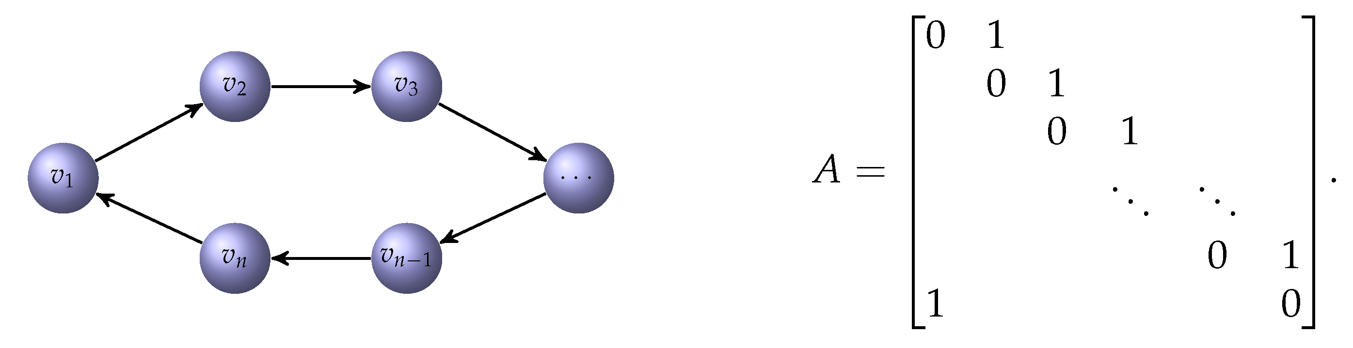
Let $A\in {\mathbb{R}}^{n\times n}$ represent the adjacency matrix of a directed circular graph. The adjacency matrix and the associated graph are displayed in Figure 2.

In this example, the matrix (16) is diagonal, with Perron root 2 of multiplicity n. In particular, the vector $\mathbf{e}$ is a Perron vector. Application of one step of the Arnoldi algorithm to the the circulant matrix A with initial vector $\mathbf{e}$ yields the eigenvector $\mathbf{e}$. Thus, the Arnoldi algorithm performs well.

Example 7.

Consider the up-shift matrix on the right-hand side of Figure 1 of order 1000. By adding the perturbation $\gamma ={10}^{-3}$ to the entry $(1000,1)$, we obtain an adjacency matrix A that represents a weighted directed circular graph. Thus, the graph is strongly connected. The associated matrix (16) is diagonal with Perron root 2 with eigenspace $span\{{\mathbf{e}}_2,{\mathbf{e}}_3,\dots ,{\mathbf{e}}_{n-1}\}$. When applying the Arnoldi algorithm to A with initial vector $\mathbf{e}$, 1000 steps are required to approximate the Perron vector. In this case, the Arnoldi algorithm performs poorly.

We conclude that the Arnoldi method may not provide useful approximations of the Perron vector of certain non-symmetric adjacency matrices A in a reasonable number of steps. The application of the Arnoldi method to A to compute the Perron vector of the matrix (16) can be competitive with the application of the Lanczos method to the latter matrix, but this is not guaranteed. The closer the adjacency matrix A is to the set of symmetric matrices, the better the Arnoldi method, applied to A, can be expected to perform.

5. Application to Real World Networks

In this section, we apply the iterative methods discussed in this paper to the computation of the Perron vector of large real-world networks, and compare the results obtained.

We start by analyzing a particular 3-chained network and seek to determine the most important vertices of each index subset according to the eigenvector centrality. Some social bookmarking services, such as Delicious, allow their users to put tags on web pages. The relationship between users, web pages and tags, can be represented by a 3-chained network [15]. A data set of Delicious bookmarks, which contains 105,000 bookmarks and 1867 users, is available at the Grouplens web site [17]. We selected data from January 2010 to February 2010 and constructed a 3-chained graph $\mathcal{G}$ with the three vertex subsets: 456 users, 4253 web pages, and 5962 tags. The total numbers of vertices and edges are 10,671 and 23,550 respectively. The 3-chained network is undirected and represented by the adjacency matrix $M\in {\mathbb{R}}^{10671\times 10671}$.

We used the power method, Lanczos iteration, and restarted the Lanczos iteration to estimate the Perron vector of M and to find the most important vertices of each vertex subset. Denote the computed approximations of the Perron vectors of M, obtained by applying the methods mentioned, by ${\mathbf{s}}_P$, ${\mathbf{s}}_L$, and ${\mathbf{s}}_{RL}$, respectively. Let the initial vector be $\mathbf{e}$ and the tolerance be ${10}^{-10}$ for all the methods. To estimate the accuracy of the methods, we consider as exact the principal eigenvector ${\mathbf{s}}_{\mathrm{exact}}$ of M computed by the built-in function eigs from MATLAB.

Before determining the most important vertices, we first check the accuracy of the approximations of the Perron vector of M computed by the above mentioned methods. We calculate the error, that is, the 2-norm of the difference between each computed approximation of the Perron vector and ${\mathbf{s}}_{\mathrm{exact}}$. The errors of the estimated Perron vectors are $0.3461$ for the power method $3.22\times {10}^{-5}$ for Lanczos iteration, and $6.69\times {10}^{-8}$ for restarted Lanczos iteration. From the errors, we observe that the Ritz vector obtained from the restarted Lanczos method is the most accurate estimator. The Ritz vector from the Lanczos algorithm is moderately accurate, while the vector found by the power method is fairly different from the exact Perron vector ${\mathbf{s}}_{\mathrm{exact}}$.

Let us now look at the performances of each method for finding the most important vertices in the three subsets “users”, “web pages” and “tags”. The results determined by the above methods and the number of iterations required are displayed in

Table 1. The most important vertices found by the methods discussed for each vertex set, and the number of iterations required by each method.

	Built-In	Power	Lanczos	ResLanc${}_{10}$
“users”	142	142	142	142
“web pages”	1368	1368	1368	1368
“tags”	4796	4796	4796	4796
iterations		34	17	3

. The most important vertices determined by ${\mathbf{s}}_{\mathrm{exact}}$ are displayed in the “Built-in” column. All of the methods identify the vertices $v_{142}$, $v_{1368}$ and $v_{4796}$ as the most important user, web page and tag, respectively. The last row, “iterations”, shows that the standard Lanczos method requires 17 matrix–vector product evaluations with A. For the restarted Lanczos, labeled ResLanc, 10 Lanczos steps are performed between each restart. Thus, it requires in this case 30 matrix–vector products. The power method requires the largest number of matrix–vector products. The rate of convergence of the approximation of the Perron vector of M computed by the Lanczos method is faster than those of the other two methods. The Ritz vector of the restarted Lanczos iteration converges more slowly but the computations require less storage space.

To better understand the numerical performance of the methods, we applied them to six undirected networks of different sizes. They are listed, together with their number of nodes, in the first column of

Table 2. Number of matrix–vector product evaluations required by the methods to reach convergence.

Network	Size	Power	Lanczos	Lanczos2	ResLanc${}_{10}$	ResLanc${}_5$
autobahn	1168	163	29	53	60	85
ndyeast	2114	1029	27	53	60	80
power	4941	49	18	35	30	35
geom	7343	19	11	23	20	20
delicious	10,671	35	17	33	30	30
internet	22,963	35	12	25	30	25
facebook	63,731	41	13	27	30	25

:

autobahn

describes the German highway system network; it is available at [18].

ndyeast  

models the protein interaction network for yeast. The data set was originally included in the Notre Dame Networks Database and is available at [19].

power      

is a representation of the U.S.A. western states power grid; see [20]. It can be found at [21].

geom        

is a weighted graph, extracted from the Computational Geometry Database geombib by B. Jones (version 2002) and is available at [19]. The entry $(i,j)$ of the adjacency matrix is the number of papers coauthored by authors i and j.

internet

is a snapshot of the structure of the Internet at the level of autonomous systems, created by Mark Newman from data for 22 July 2006 [21].

facebook

describes the friendship links of the New Orleans Facebook network resulting from a particular snapshot. The dataset was studied in [22] and is available at [23].

Table 2 displays the number of matrix–vector product evaluations carried out by the methods considered to reach convergence. We also report the results obtained for the delicious network for comparison. The label Lanczos2 denotes the results obtained by Algorithm 2, that is, by applying the Lanczos recursion twice to save storage space. In this case, the number of matrix–vector product evaluations is roughly twice the number of iterations required by the standard algorithm (Algorithm 1) if the stopping criterion is adjusted to produce the same accuracy in the approximation of the Perron vector. The restarted Lanczos method (ResLanc) was executed with both ten and five iterations between each restart, so the number of matrix–vector product evaluations is obtained by multiplying the number of iterations by ten and five, respectively. For the other methods, the number of matrix–vector product evaluations coincides with the number of iterations.

Table 3. Errors produced by the methods with respect to the Perron vector computed by the eigs function of MATLAB.

Network	Size	Power	Lanczos	Lanczos2	ResLanc${}_{10}$	ResLanc${}_5$
autobahn	1168	$1.09\times {10}^{-3}$	$7.62\times {10}^{-5}$	$2.42\times {10}^{-4}$	$9.60\times {10}^{-6}$	$7.46\times {10}^{-5}$
ndyeast	2114	$1.47\times {10}^{-2}$	$7.96\times {10}^{-5}$	$7.96\times {10}^{-5}$	$2.37\times {10}^{-6}$	$7.59\times {10}^{-5}$
power	4941	$2.76\times {10}^{-4}$	$3.66\times {10}^{-5}$	$3.66\times {10}^{-5}$	$9.77\times {10}^{-8}$	$8.18\times {10}^{-6}$
geom	7343	$1.66\times {10}^{-5}$	$6.53\times {10}^{-6}$	$1.28\times {10}^{-6}$	$2.60\times {10}^{-10}$	$5.10\times {10}^{-8}$
delicious	10,671	$3.46\times {10}^{-1}$	$3.22\times {10}^{-5}$	$3.22\times {10}^{-5}$	$6.73\times {10}^{-8}$	$5.42\times {10}^{-6}$
internet	22,963	$6.77\times {10}^{-5}$	$3.15\times {10}^{-5}$	$8.97\times {10}^{-6}$	$1.51\times {10}^{-11}$	$2.36\times {10}^{-7}$
facebook	63,731	$9.74\times {10}^{-5}$	$2.37\times {10}^{-5}$	$6.86\times {10}^{-6}$	$2.38\times {10}^{-10}$	$1.05\times {10}^{-6}$

reports the 2-norm errors for each method. The Perron vector returned by the function eigs of MATLAB is considered the exact vector.

We see that the power method requires more iterations than the Lanczos algorithm (Algorithm 1) and delivers approximations of the Perron vector of worse accuracy. Applying the Lanczos method twice by Algorithm 2 saves storage but results in a heavier computational load in order to produce the same accuracy of the computed approximation of the Perron vector. The restarted Lanczos approach has the remarkable feature of requiring the same number of matrix products when it is executed, performing ten and five iterations between consecutive restarts. This means that just a few iterations are sufficient to guarantee convergence. The computer storage requirement is much smaller than for the Lanczos method. The errors in the computed approximations of the Perron vector achieved by the restarted Lanczos method are smaller than the errors obtained with the Lanczos methods (Algorithms 1 and 2). Table 2 indicates that the restarted Lanczos method can be competitive.

6. Conclusions

This paper compares the computational effort and storage requirements of the power method, Lanczos method, and the restarted Lanczos method to determine the Perron vector for a large symmetric adjacency matrix. The application of the Arnoldi iteration is also considered. The power method yields quite a slow convergence, much slower than that of the Lanczos method. However, due to its large storage requirement for large adjacency matrices, the latter method is not practical to use for large-scale networks. Different ways of restarting the Lanczos iterations are considered and found to combine faster convergence than the power method with less storage requirement than the Lanczos method.

References

- Estrada, E. The Structure of Complex Networks: Theory and Applications; Oxford University Press: Oxford, UK, 2012. [Google Scholar]
- Newman, M.E.J. Networks: An Introduction; Oxford University Press: Oxford, UK, 2010. [Google Scholar]
- Brandes, U. A faster algorithm for betweenness centrality. J. Math. Sociol. 2001, 25, 163–177. [Google Scholar] [CrossRef]
- Kleinberg, J.M. Authoritative sources in a hyperlinked environment. J. ACM 1999, 46, 604–632. [Google Scholar] [CrossRef]
- Bonacich, P. Power and centrality: A family of measures. Am. J. Sociol. 1987, 92, 1170–1182. [Google Scholar] [CrossRef]
- Meyer, C.D. Matrix Analysis and Applied Linear Algebra; SIAM: Philadelphia, PA, USA, 2000. [Google Scholar]
- Estrada, E.; Knight, P.A. A First Course in Network Theory; Oxford University Press: Oxford, UK, 2015. [Google Scholar]
- Blondel, V.D.; Gajardo, A.; Heymans, M.; Senellart, P.; Van Dooren, P. A measure of similarity between graph vertices: Applications to synonym extraction and web searching. SIAM Rev. 2004, 46, 647–666. [Google Scholar] [CrossRef]
- Bondy, J.A.; Murty, U.S.R. Graph Theory with Applications; Macmillan: London, UK, 1976. [Google Scholar]
- Concas, A.; Noschese, S.; Reichel, L.; Rodriguez, G. A spectral method for bipartizing a network and detecting a large anti-community. J. Comput. Appl. Math. 2020, 373, 112306. [Google Scholar] [CrossRef] [Green Version]
- Concas, A.; Fenu, C.; Rodriguez, G. PQser: A Matlab package for spectral seriation. Numer. Algorithms 2019, 80, 879–902. [Google Scholar] [CrossRef] [Green Version]
- Saad, Y. Numerical Methods for Large Eigenvalue Problems, 2nd ed.; SIAM: Philadelphia, PA, USA, 2011. [Google Scholar]
- Bapat, R.B. Graphs and Matrices; Springer: London, UK, 2010. [Google Scholar]
- Concas, A.; Reichel, L.; Rodriguez, G.; Zhang, Y. Chained graphs and some applications. Appl. Netw. Sci. 2021, 6, 39. [Google Scholar] [CrossRef]
- Ikematsu, K.; Murata, T. A fast method for detecting communities from tripartite networks. In Proceedings of the International Conference on Social Informatics, Kyoto, Japan, 25–27 November 2013; Springer: Cham, Switzerland, 2013; pp. 192–205. [Google Scholar]
- CITESEERX, Computer and Information Science Papers. CiteSeer Publications ReserchIndex. Available online: https://citeseerx.ist.psu.edu/index (accessed on 5 May 2021).
- Grouplens. Available online: https://grouplens.org/datasets/hetrec-2011 (accessed on 5 May 2021).
- Biological Networks Data Sets of Newcastle University. Available online: http://www.biological-networks.org/ (accessed on 5 May 2021).
- Batagelj, V.; Mrvar, A. Pajek Data Sets. Available online: http://vlado.fmf.uni-lj.si/pub/networks/data/ (accessed on 5 May 2021).
- Watts, D.J.; Strogatz, S.H. Collective dynamics of ‘small-world’networks. Nature 1998, 393, 440–442. [Google Scholar] [CrossRef] [PubMed]
- Mark Newman’s Web Page. Available online: http://www-personal.umich.edu/~mejn/netdata/ (accessed on 5 May 2021).
- Viswanath, B.; Mislove, A.; Cha, M.; Gummadi, K.P. On the evolution of user interaction in Facebook. In Proceedings of the 2nd ACM Workshop on Online Social Networks (WOSN’09), Barcelona, Spain, 17 August 2009; pp. 37–42. [Google Scholar]
- The Max Plank Institute for Software Systems. Available online: http://socialnetworks.mpi-sws.org/data-wosn2009.html (accessed on 5 May 2021).
Figure 1.
A directed graph and its adjacency matrix A.
Figure 2.
A directed circular graph and its adjacency matrix A.