Heat Exchanger Network Retrofit of an Oleochemical Plant through a Cost and Energy Efficiency Approach

Abstract

Limited research of heat integration has been conducted in the oleochemical field. This paper attempts to evaluate the performance of an existing heat exchanger network (HEN) of an oleochemical plant at 600 tonnes per day (TPD) in Malaysia, in which the emphases are placed on the annual saving and reduction in energy consumption. Using commercial HEN numerical software, ASPEN Energy Analyzer v10.0, it was found that the performance of the current HEN in place is excellent, saving over 80% in annual costs and reducing energy consumption by 1,882,711 gigajoule per year (GJ/year). Further analysis of the performance of the HEN was performed to identify the potential optimisation of untapped heating/cooling process streams. Two cases, which are the most cost-effective and energy efficient, were proposed with positive results. However, the second case performed better than the first case, at a lower payback time (0.83 year) and higher annual savings (0.20 million USD/year) with the addition of one heat exchanger at a capital cost of USD 134,620. The first case had a higher payback time (4.64 years), a lower annual saving (0.05 million USD/year) and three additional heaters at a capital cost of USD 193,480. This research has provided a new insight into the oleochemical industry in which retrofitting the HEN can further reduce energy consumption, which in return will reduce the overall production cost of oleochemical commodities. This is particularly crucial in making the product more competitive in its pricing in the global market.

1. Introduction

Being one of the largest exporters of palm oil and its associated products, Malaysia provides approximately 20% of the world’s production of oleochemicals [1]. As recently as 2018, there were 19 oleochemical plants operating in Malaysia, producing approximately 2.7 million tons of oleochemicals annually [2]. Modern-day industrial oleochemical production involves complex reactions and energy-intensive processes, utilising heavy-duty industrial equipment such as boilers and special separation towers. The world energy consumption is projected to rise nearly 50% from 600 to almost 900 quadrillion British thermal units (BTU) between 2018 and 2050 with the industrial sector as the largest consumer, constituting more than half of the share [3]. Meanwhile, the industrial sector in Malaysia used 29.5% or 19,046 kilotonnes of oil equivalent (ktoe) of the final energy demand in 2018 [4], in which many of the fuels are derived from non-renewable sources. According to some published literature, the fuels that are often involved are non-renewable; hence, they will be inevitably exhausted in 40 years or four centuries, depending on the information source [5].

While great strides have been made in the search for renewable alternatives, conventional energy sources are still forecasted to account for about 78% of the global energy consumption in 2040 [6]. The ventures in finding alternatives sources remain ongoing; therefore, so must the task of prolonging conventional energy sources, until their alternatives are ready for global-scale implementation. Heat integration (HI) has been one of the effective ways of managing these resources. It is a thermodynamics-based approach to minimise energy consumption of process streams by calculating the feasible energy targets. In modern plants, a series of heat exchangers are constructed according to a pre-fixed production rate which is optimised through heat integration. However, as demand for oleochemicals and other commodities continues to grow, industries would need to alter their production rates or expand existing facilities, compromising the formerly optimised heat exchanger network (HEN). In such cases, a retrofit of an existing HEN can be considered to eliminate or minimise the increase in energy consumption from the change in production rate. The retrofit design, defined as “modification to an existing plant to improve its performance”, could be evaluated in the terms of the reduction in energy consumption, utility costs, or other variables [7]. These endeavours in HEN retrofits can typically achieve a reduction in hot and cold utilities by up to 40% compared with original designs or existing installations [7]. Other motives behind a retrofit project include the permanent change in feed/product specifications, increase in demand which is significant enough to increase production rate (but insufficient to construct a new plant), improving safety, and reducing waste emissions [7]. Much work has been done in the olefin industry, as listed in

Table 1. Recent studies in heat exchanger network retrofits and their results.

Industry	Annual Energy Saving	Annual Operating Cost Saving (USD)	Capital Investment (USD)
Ethylene plant [8]	-	3.05 million	3.87 million
Fluid catalytic cracking [9]	27%	-	-
Ethylene plant [10]	5.6%	0.61 million	0.71 million
Petroleum refinery [11]	34%	149,954	1.5 million

below.

Meanwhile, there are also other reported studies using HI implementation such as the brewing industry [12], pulp and paper industry [13], beet sugar [14], and oil refineries [15]. The main outcome of this study is meant to reduce energy saving while maintaining or improving the yield of production.

Table 2. Cost savings and payback time for industries.

Industry	Cost Savings	Payback Time
Petrochemical	30% of imported fuel Improved co-generation	12–24 months
Inorganics	30% of total energy	9–16 months
Chemicals	30% of total energy	15 months
Pharmaceuticals	20–40% of total energy	2–2.5 years
Resins	25% + debottlenecking	Up to 3 years
Pigments	15% of total energy	15 months
Steelworks	50% increase in power generation	2 years
Foodstuffs	25% of total energy	2 years

below shows impressive cost savings and payback times from HEN implementation in various industries 20 years ago [10]. This shows that HEN can create great impacts to industrial sector because it provides continuous operating cost saving and low risks of investment return.

As seen in Table 1 and Table 2 above, little has been written about HEN retrofits in the oleochemical industry at the time of writing, despite the industry being renowned for its high energy requirement. Recent literature of HI in oleochemical industry includes utilising waste heat from boilers [16], and the retrofit of a dividing wall column for oleochemical separation [17].

Therefore, because the literature regarding HEN retrofit in the oleochemical industry is limited, this paper seeks to contribute to the present information and address the gap. The retrofit approach has allowed for evaluation to be performed and improvement for the existing HEN to be investigated. We hope that the paper further serves as a great inspiration to other industrial players in the field to consider implementation and retrofits of HENs in their respective fields. Lastly, this paper aims to serve as a blueprint for future oleochemical plant design and energy management evaluation.

2. Methodology

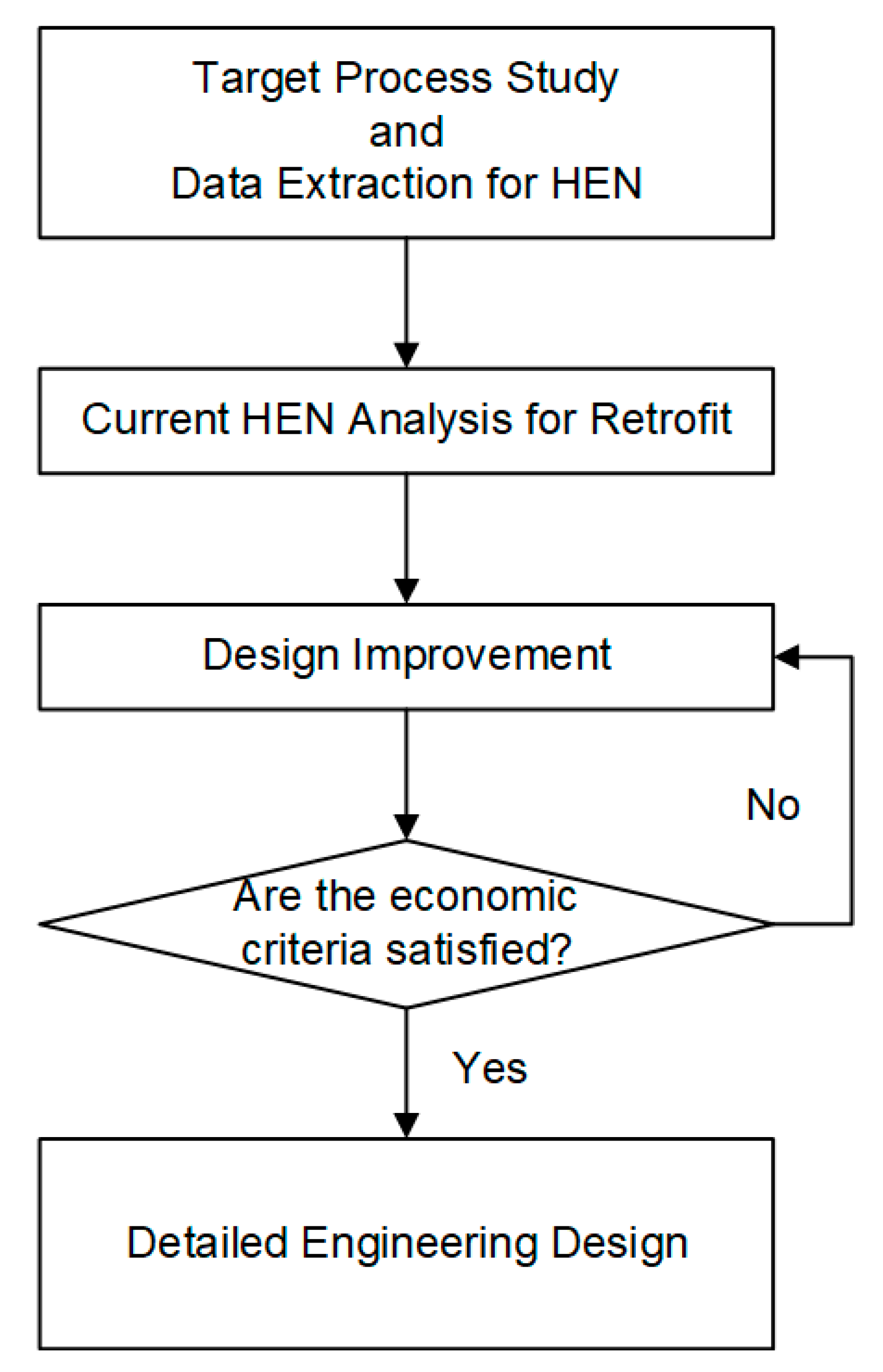
The procedure for HEN retrofit of an existing plant was inspired and modified from the work produced by Yoon et al. [10]. The summary of the methodology can be seen in the illustration in Figure 1 below. The first step towards retrofitting is to understand the boundaries of the process that takes place and to correctly extract relevant data. The process stream data such as temperature across the process stream, utilities’ properties, and so forth are crucial to obtain the necessary energy absorbed or rejected for HEN design. Subsequently, energy requirements for each stream are evaluated, and heat integration can be performed using the standard rule of thumb for stream matching. Linnhoff and Hindmarsh [18] provided a detailed guide for pinch analysis. From the study, the main criteria for any amendment of HEN improvement are based on its improved economic returns. The trade-offs between capital investment and annual operating cost, the payback period, will be used as the main pointer for HEN system design improvement. Process streams are classified as either hot or cold, with the hot streams being responsible for supplying energy to cold streams. The asterisk signs next to the streams indicate that a phase change has occurred. This research was initiated upon receiving both process stream data and corresponding utilities data in

Table 3. Stream process data.

Stream	Process	Utility Required (kW)	Initial Temperature (°C)	Final Temperature (°C)
A	Cooling	1035	175	90
B	Cooling	477	90	50
C	Cooling	256	118	50
D *	Cooling	15,307	220	82
E *	Cooling	14,690	216	83
F *	Cooling	2348	130	130
G	Heating	1035	60	116
H	Heating	1499	127	240
I	Heating	2290	203	232
J	Heating	81	75	134
K	Heating	2104	82	220
L	Heating	85	50	100
M *	Heating	12,715	83	216
N *	Heating	17,282	49	203
O *	Heating	2348	65	103
P *	Heating	163	73	102
Q	Heating	965	203	228

* Refers to stream that will undergo a phase change process.

and

Table 4. Utilities used and their properties.

Utilities	Temperature In (°C)	Temperature Out (°C)	Pressure (barg)	Cost (USD/kJ)
Cooling Water	34	40	6	4.50 × 10−8
Tempered Water	55	65	5	4.10 × 10−7
Low Pressure Steam	144	144	3	1.16 × 10−5
Medium Pressure Stream	175	175	8	1.10 × 10−5
Hot Oil	280	260	5	7.80 × 10−6

, respectively.

Information relating to other properties of the process fluids were not shown for confidentiality reasons. Natural gas prices for industrial uses in Malaysia in 2020 as given by Gas Malaysia [19] were subjected to the consumption volume. In this paper, the tariff taken was USD 8.19 per million British thermal units (MMBTU) for a minimum monthly consumption of 62,500 MMBTU. Properties of DOWTHERM Q [20] were taken to be the properties of hot oil in this study. The cost of steam generation (for medium pressure (MP) and low pressure (LP) steam) was adapted from the U.S. Department of Energy [21], with an assumed boiler efficiency of 0.8. The cost for operating a cooling tower is approximately 0.13 USD per kilowatt (kW) per 100 feet of head per 1000 gallons of water pumped [22]. The electrical tariff for industrial use was taken at 0.049 USD per kW [23]. This study assumed the height of cooling towers to be 100 feet, and 97 wt.% of water was reused in the cooling tower while the remaining 3 wt.% was evaporated during the tower cooling process [24]. The makeup water was obtained from the state’s water provider. In Malaysia, water tariffs differ through the type of supply (domestic or non-domestic), state, and minimum monthly consumption [25]. In this study, it was assumed that a minimum monthly quota of 35 m³ was consumed, and because the water used in this study was for industrial purposes and the plant was located in Selangor, the cost of makeup water as 0.55 USD per m³ [25]. The costs of utilities were provided by the industry partner and were used to calculate the payback time.

With 10 °C as the log mean temperature difference (LMTD) for heat transfer, the stream matching process could take place with great aid of a numerical tool, ASPEN Energy Analyzer (AEA). The demonstration of AEA can be found in the supplementary material (Appendix B) using a simple case study. The current study consisted of two objectives:

• To evaluate current plant’s HEN performance;
• To retrofit the plant HEN based on two goals:
  • Become the most energy-efficient;
  • Become the most cost-efficient.

Economic analysis for each case is investigated to determine trade-offs between energy savings and capital investment. Once a desired retrofit design is chosen, detailed engineering design proceeds.

The next section will start with the evaluation of an HEN without any heat integration in place (Case 0) and is followed by an evaluation of the current HEN in place (Case 1). Results from Case 0 provide an insight on the high energy and operational cost required for an oleochemical plant without the assistance of HI. Then, Case 1 details how HI functions as an effective energy management tool as compared to Case 0. Subsequent cases (Cases 2 and 3) are retrofit proposals based on the two goals, which are the most energy-efficient and the most cost-efficient approach.

3. Results and Discussion

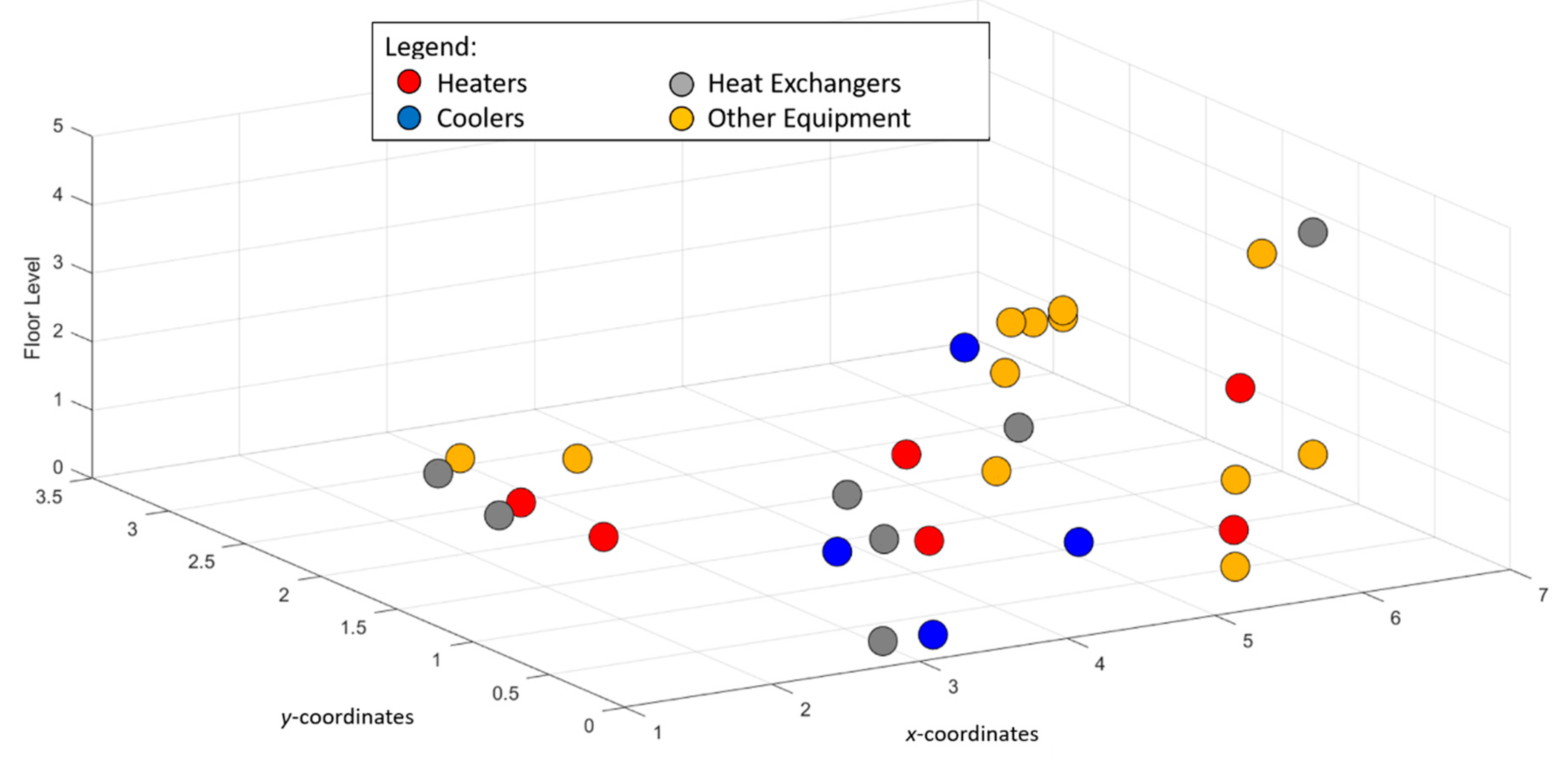
The current plant layouts for all heat exchangers, heaters, and coolers for cold and hot streams were mapped using a 3D MATLAB plot, as shown in Figure 2 below. The HEN was constrained within a dimension of 85 m length by 45 m width by 55 m height. There were six heaters, four coolers, and seven heat exchangers in this section of the plant. Floor level 0 and floor level 5 represent the ground floor and the highest floor, respectively. In Figure 2 below, “Other Equipment” refers to heaters/coolers/heat exchangers irrelevant to this study, although are included in the footprint as a visual representation of the limited space in this plant. Here, the complexity of the HEN becomes more apparent. The locations for the heating and cooling equipment are scattered throughout the plant, while the main unit operations are compacted within the plant, which are not shown here due to confidentiality. Minimal changes are highly desired from the industry to avoid possible complications arising from extreme modifications. Furthermore, the limited available space has to be conserved for personnel safety in accordance with safety guidelines and any other future remodelling possibilities. The MATLAB coding for the utilities’ coordinates can be found in the supplementary material (Appendix A). Subsequent cases (suggestion for the placement of new equipment for Case 2 and Case 3) can also be found under the same section.

3.1. Case 0—Benchmark

Case 0 is the benchmark case where no heat exchangers are utilised for energy integration. Only utilities are allowed for heating and cooling requirements. Case 0 provides an overview of the energy-demanding operation of an oleochemical production facility. All present-day plants have some form of HEN in place, except in cases where space is limited (e.g., offshore oil and gas platforms). Evaluation of a base case may appear pointless because no modern chemical plants operate without an HEN, but this evaluation provides a numerical finding of how energy-intensive an oleochemical process plant can be.

Table 5. Results for Case 0.

Stream	Process	Utility Required (GJ/Year)	Initial Temperature (°C)	Final Temperature (°C)	Utility	Operating Cost (USD/Year)
A	Cooling	29,808	175	90	Tempered Water	12,240
B	Cooling	13,738	90	50	Cooling Water	620
C	Cooling	7372	118	50	Cooling Water	333
D	Cooling	440,842	220	82	Tempered Water	181,016
E	Cooling	423,072	216	83	Tempered Water	173,719
F	Cooling	67,622	130	130	Tempered Water	27,767
G	Heating	32,486	60	116	LP Steam	375,658
H	Heating	43,171	127	240	Hot Oil	335,136
I	Heating	65,940	203	232	Hot Oil	511,889
J	Heating	2343	75	134	LP Steam	27,092
K	Heating	60,584	82	220	Hot Oil	470,313
L	Heating	2447	50	100	LP Steam	28,294
M	Heating	366,192	83	216	Hot Oil	2,842,736
N	Heating	497,722	49	203	Hot Oil	3,863,795
O	Heating	67,622	65	103	LP Steam	781,955
P	Heating	27,782	203	228	Hot Oil	215,668
Q	Heating	4694	73	102	LP Steam	54,284
Sum		2,153,437				9,902,515

summarises the utilities used and required by the streams, with the respective operating costs.

From Table 5, the stream with the lowest cold utility requirement (stream C) also has the lowest annual operating cost (333 USD/year). On the other hand, the stream with the lowest hot utility requirement (stream L) operates at 28,294 USD/year, a factor 85-fold greater than stream C. A deduction can be made that greater savings in heating utility produce greater savings in heating cost, in contrast to a cooling utility. Upon further observation, while the total utility required and the operating cost exceeded two million GJ and nine million USD yearly, it can be seen that there is a great divide between the energy and cost required between the phase change streams and non-phase change streams. The energy consumed and operating cost by phase change streams (1,890,854 GJ/year and 8,086,655 USD/year) is significantly higher than the non-phase change streams (262,583 GJ/year and 1,815,859 USD/year).

As discussed, large modifications are discouraged to avoid adverse results in practice. Overall, the hot and cold utility requirements for phase change streams are equal at 931,536 GJ/year. Theoretically, through pinch technology, no external utilities are required for these streams. In Case 0, the hot and cold process streams undergoing phase change are fully integrated with each other, and provide significant savings to the system. Furthermore, there are safety hazards associated with streams undergoing phase change. Thus, modification proposals (Cases 2 and 3) will not consider the phase change streams except for stream P, because the low utility and operating cost stream is considered as a low-risk stream to be retrofitted. To reiterate, this section of this journal aims to showcase the scale of energy and cost required to operate an oleochemical plant. Case 0 has effectively demonstrated its objective by calculating the astronomical energy and cost required annually. Significant savings in energy and cost are expected in Case 1, which is a recreation of the current setup. After that, Case 1 will be re-evaluated. Two retrofit cases are proposed; one is constrained by minimal additional cost (Case 2) and the other is focused on maximum energy recovery (Case 3).

3.2. Case 1—Current Case

The current HEN is reproduced below in Figure 3. It underwent heat integration by the industrial partner several years prior to this research and has been in place ever since. Case 1 was evaluated with Case 0 to investigate the energy saved in an existing oleochemical plant. Findings from this will be a valuable addition to the limited data available in the oleochemical industry. The simulation in AEA produced results that matched data provided by industrial partner. Replication of an HEN is feasible in AEA; therefore, the streams were deemed suitable to undergo retrofitting using the software. The performance of the current HEN was investigated and compared with its base case in terms of energy and operating cost reduction.

Due to multiple utilities, there were two series of hot and cold pinches, which are 144 °C and 134 °C as well as 70 °C and 60 °C, when using an LMTD of 10 °C. The same temperature pinches occurred for Cases 2 and 3. There were four coolers, six heaters, and three heat exchangers in total for non-phase change streams. Compared to Case 0, the current HEN provided a total reduction of 80.82% in operating cost and 87.43% in energy consumption. However, these superficial data alone do not provide any in-depth context on streams’ interactions and how the retrofit process can be simplified henceforth.

However, following careful inspection, the current HEN restricted hot and cold phase change streams within themselves, except for stream P. Thus, two tables are presented to segregate the data.

Table 6. Results for Case 1 (non-phase change streams and stream P *, a phase change stream).

Stream	Process	Utility Required (GJ/Year)	Initial Temperature (°C)	Final Temperature (°C)	Utility	Operating Cost (USD/Year)
A	Cooling	25,114	175	90	Tempered Water	10,312
B	Cooling	11,059	90	50	Cooling Water	499
C	Cooling	4925	118	50	Cooling Water	222
G	Heating	29,808	60	116	LP Steam	328,443
H	Heating	43,171	127	240	Hot Oil	335,136
I	Heating	65,940	203	232	Hot Oil	511,889
J	Heating	2343	75	134	LP Steam	27,092
K	Heating	60,584	82	220	Hot Oil	470,313
L	Heating	-	50	100	-	-
P *	Heating	-	73	102	-	-
Q	Heating	27,782	203	228	Hot Oil	321,378
Sum		270,726				2,005,285

tabulates the data for non-phase change streams and stream P.

The overall result of the HEN in place for the non-phase change streams and stream P is promising. A cost reduction of 26,242 USD/year (0.27%) was achieved with an energy reduction of 19,639 GJ/year (0.91%). The heating requirements for stream L and P were completely eliminated, rendering their utility requirement and operating cost as zero.

As the hot and cold utilities are eliminated, the operating costs for these streams are also eliminated. The annual cost saved is 7.88 million USD/year (79.48%) and energy savings of 1,863,072 GJ/year (86.52%) were achieved, which is significantly higher the non-phase change streams. In addition to the tremendous amount of savings from these “phase change streams”, as well as the safety and operational issues, the streams mentioned formerly (D, E, F, M, N, and O) in Table 5 were excluded in Case 2 and Case 3. Excluding these streams allows the industry’s desire for minimal changes to be further fulfilled. While significant reduction in energy is achieved compared to Case 0, other opportunities are available for further heat exchange to take place, which are the 1427 kW of cooling energy and 7974 kW of heating energy. The excess cooling energy remaining indicates that heat integration is not optimised. The availability of untapped energy from the streams arose from several changes in utility demand after a few years in operation. Expanding from Case 1, two retrofit models are proposed in the subsequent sections.

3.3. Case 2—Design for Minimum Additional Cost

Case 2 allows only minor work between non-phase changing streams of the plant, allowing cost to be minimised because, theoretically, only re-piping of different streams to existing heaters, coolers, and heat exchangers (HEs) is implemented. In practice, this would be achieved through the removal of the hot and cold pipelines from the heat exchanger. Then, different hot and cold pipelines would be reinstalled on the same heat exchanger. Minimal re-piping work can be conducted within the typical downtime time frame. The only equipment involved with this retrofit is pipelines which can be reused from existing units; therefore, the cost involved in this modification process, should this retrofit process be chosen, would theoretically be low. In addition, it will not hinder the existing free space because the pipes can be relocated and angled around the plant.

The usage of MP steam was initially planned to be replaced with LP steam to reduce the operating cost of the plant. However, it was found that the reactor connected to this stream with catalysts in place undergoes frequent deactivation; hence, MP steam is required to increase the stream temperature to 20–30 °C higher than its normal operating conditions to reactivate the catalysts. For this reason, MP steam remains the utility for stream G. The results of Case 2, which can be seen in Figure 4 below, outline a recreated network for the heat exchange process within the plant where streams D*, E*, M*, N*, and O* remain untouched.

As seen in Figure 4, there are four coolers, nine heaters and three heat exchangers after retrofitting this HEN following from Case 1. There was no new heat exchanger used because all heat exchangers from A, B, and C were re-used in their respective streams. Unexpectedly, there were three additional heaters in this retrofit design, even though the condition set only allowed for re-piping modifications. When reassigning the existing heaters, coolers and HEs to different streams, the heating requirements of streams K, L, and P were left unfulfilled because all the pre-existing equipment was in place with other streams. Hence, three heaters were added to ensure the necessary heating process took place. At first glance, although the results produced from this case required only three additional heaters (which may appear insignificant at first), this section of the plant already had 13 equipment in place. Furthermore, the addition of three heaters required at least three pumps or compressors for their respective utilities. Despite this unexpected outcome, the overall performance of Case 2 was positive because there were reductions in utility consumption and their operating costs, as seen in

Table 7. Results for Case 2.

Stream	Process	Utility Required (GJ/Year)	Initial Temperature (°C)	Final Temperature (°C)	Utility	Operating Cost (USD/Year)
A	Cooling	18,922	175	90	Tempered Water	7769
B	Cooling	6883	90	50	Cooling Water	311
C	Cooling	6883	118	50	Cooling Water	311
G	Heating	26,381	60	116	MP Steam	305,060
H	Heating	43,171	127	240	Hot Oil	335,138
I	Heating	65,952	203	232	Hot Oil	511,985
J	Heating	2333	75	134	LP Steam	26,976
K	Heating	49,709	82	220	Hot Oil	385,889
L	Heating	1958	50	100	LP Steam	22,646
P *	Heating	4694	203	228	Hot Oil	36,443
Q	Heating	27,792	73	102	LP Steam	321,378
Sum		254,678				1,953,906

. It could be expected that this retrofit required a high capital expenditure. While there seems to be much more energy to be extracted (1135 kW cold and 6792 kW hot), another potential stream matching was not possible due to the temperature crossing of streams. As an example, the stream is shown in the supplementary material (Appendix B).

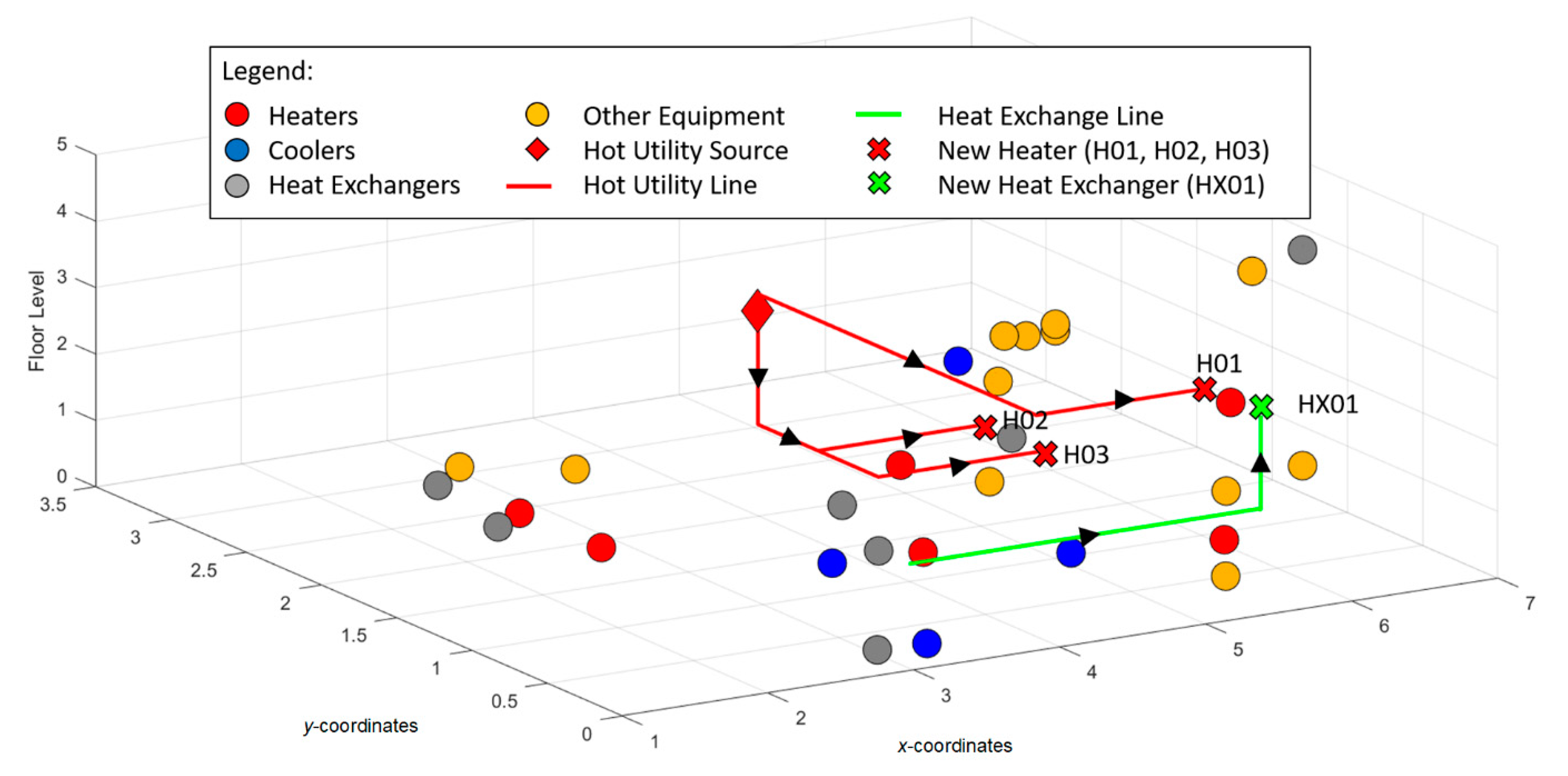
Figure 5 below shows the visual representation for the suggestion of possible modification work for Case 2. The three new heaters and one new heat exchanger are labelled as H01, H02, H03, and HX01, respectively. HX01 is the existing heat exchanger between stream A and P from the Case 1, which is repositioned to be between streams A and K. The arrangement of the new heaters and heat exchanger are set in proximity (approximately 2 m) with the existing equipment in-line with the streams.

The overall cost of operation dropped by 51,380 USD yearly (2.56% based on Case 1), and there was an energy reduction of 16,057 GJ yearly (5.93% based on Case 1). This, however, comes at the expense of new heaters and the minor equipment (pump and compressor), as well as modification operations such as re-piping work. Calculations were performed through an equation-based cost model for a shell and tube heat exchanger based on the heat transfer area from a U.S. Department of Energy proposal [26].

Table 8. Heaters’ area and costs for Case 2.

Stream	Area (m2)	Cost
		(USD)
G	18.78	68,309
K	19.64	68,588
P *	4.92	63,814
Sum	43.35	200,711

summarises the costs for the heaters required for this retrofit to take place.

3.4. Case 3—Design for Maximum Heat Recovery

While Case 2 minimises major changes and focus more on minor changes (e.g., re-piping process streams), Case 3 aims to minimise major changes through the addition a new heat exchanger. Case 3 introduces one or more heat exchanger between a hot and cold stream with the highest energy saving potential, thus reducing their dependency on the central utility system.

Figure 6 summarises the available heating and cooling potential from the existing plant. There were three hot streams and six cold streams which had a potential of 1329 kW of cooling energy and 7974 kW of heating energy. While in theory, all 1329 kW of the cooling energy could be integrated in the hot streams, as in Case 2, this is not feasible due to pinch temperature crossing.

Eliminating the hot streams (A, B, and C) first is counterintuitive, because there are more cold streams that hot streams. Eliminating hot streams is performed because it allows the most suitable hot stream to be the determinant for stream matching. Stream A had the highest cooling energy available (872 kW) and the highest driving force (85 °C). Stream B had the second highest cooling energy available (384 kW) and the second highest driving force (40 °C). Stream C had the two lowest cooling energies available (128 kW and 43 kW), and also the lowest driving forces (34 °C and 11 °C). Stream A had the highest potential for the hot stream in this retrofit project.

A weightage table,

Table 9. Weight table for Case 3.

Stream	Available Energy		Driving Force		Overall Weight
	(kW)	Weight	(°C)	Weight
G	1035	4	56	4	4
H	1499	3	113	2	2.5
I	2290	1	29	5	3
J	81	6	59	3	4.5
K	2104	2	138	1	1.5
Q	965	5	25	6	5.5

, was made to facilitate the decision-making process for the cold streams. The weight value 1 for parameters “Available Energy (kW)” and “Driving Force (°C)” indicates the greatest available energy and driving force available. The overall weight was the average of the two individual weight values. Hence, a lower overall weight value indicates a higher driving force and available energy, which proposes better suitability to be matched with hot stream A.

From the table, stream K has the highest overall weight; hence, it was chosen for stream matching with stream A, and the HEN is illustrated in Figure 7.

Heat exchange takes place between a single hot and cold stream and saves 872 kW per stream (total of 1744 kW). The operating and energy expenditure from this retrofit are reduced by 205,270 USD/year and 50,227 GJ/year. As in Case 2, there is some energy that can be potentially saved (675 kW of cooling energy and 7102 kW of heating energy). However, similarly to its predecessor, temperature cross occurs again between the hot and cold streams, as seen in the supplementary material (Appendix B.4). Here, a greater cost reduction in hot oil as compared to tempered water is observed because the cost of the heating medium (due to consumption in fuel) is higher than the cooling medium which undergoes the relatively lower operating cost cooling process in the cooling tower.

Figure 5 above shows a suggestion for the heat exchanger placement for Case 3. As with Case 2, the heat exchanger is given the name HX01. HX01 from Case 2 is an existing heat exchanger of stream A (repositioned to match stream K from stream P). However, in Case 3, HX01 is a new heat exchanger. As in Case 2, HX01 is repositioned to be as close as possible to the existing equipment in-line with the stream. Additionally, HX01 from Case 2 and Case 3 undergoes heat exchanges of 387 kW and 872 kW, respectively.

Using the same method proposed by Kim et al. [26] and a 15% addition from modification works, the cost and the area of the heat exchanger are presented in

Table 10. Heat exchanger area and cost for Case 3.

Streams	Area (m2)	Cost (USD)
G and K	238.81	139,650

.

The return of investment (ROI) for this case is 10 months at a capital cost of USD 139,650. The next section of this paper will balance the capital cost, operational expenditure, and other financial considerations of Case 2 and Case 3.

3.5. Detailed Cost Analysis and Recommendation

Table 11. Evaluation of Cases 1, 2 and 3.

Pathways	Case 1	Case 2	Case 3
No. of Appliances	17	20	18
Heaters	6	9	6
Coolers	4	4	4
Heat Exchangers	7	7	8
Utilities	Cooling Water	Cooling Water	Cooling Water
	Tempered Water	Tempered Water	Tempered Water
	LP Steam	LP Steam	LP Steam
	MP Steam	MP Steam	MP Steam
	Hot Oil	Hot Oil	Hot Oil
Utility Required (GJ/year)
Hot	229,638	221,990	204,524
Cold	41,098	32,688	15,984
Total	270,736	254,678	220,508
Annual Cost (million USD/year)
Heating	1.99	1.94	1.80
Cooling	0.0120	0.0072	0.0005
Total	2.00	1.95	1.80
Total Utility Saved Based on Case 1
(GJ/year)	-	16,057	50,227
(% GJ/year)	-	5.93	18.55
Annual Savings Based on Case 1
(million USD/year)	-	0.05	0.20
Modifications
Equipment Size (m2)	-	43.35	238.81
Equipment Cost (USD)	-	193,456	134,602
Associated Piping and Insulation Cost (USD)	-	29,018	20,190
Total Cost (USD)	-	222,474	154,792
Economic Return
Payback Time (year)	-	4.64	0.83
Return on Investment (ROI) (%)	-	7.72	535

below summarises the performance of the current HEN (Case 1) and the modification requirements of the retrofit projects (Case 2 and Case 3). The ROI was calculated based on a five-year period, because the plant may require another possible retrofit after the end of this the time frame. The cost of piping for a 3” Schedule 5 SS316 was taken to be 14.09 USD/metre [27]. The cost associated with piping and insulation was assumed to be 15%. The demonstrations of Case 2 and Case 3 were merely on pipe length. The addition of capital investment such as valves, compressors, pumps, and other accessories are subject to plant constraint and the industrial partner’s interests.

The modifications made in Case 3 showed a better overall return for the plant. In Case 2, while the total heat transfer area (43.35 m²) was lower than Case 3 (238.81 m²), this did not translate to a lower capital cost because there were three new heaters needed for the plant. To reiterate, Case 2 was designed to minimise additional cost by undergoing minor re-piping works, to perform better economically. However, additional heaters were added due to unfulfilled heating requirements after stream re-matching was performed, leading to higher capital expenditure. This still produced positive but less satisfactory results compared to Case 3. Due to the lower annual operating cost saved, the payback time for Case 2 was also higher than Case 3. Subsequently, the ROI of Case 2 after five years was lower than Case 3, because it had just finished its payback period a short time before. Case 3 had a lower operating cost than its annual operation expenditure (OPEX) saved; therefore, the payback period was less than a year. Consequently, the ROI over five years was more than 500%.

Both retrofit routes presented in this study produced positive feedbacks. Given that a retrofit HEN project is an open-ended venture and both Case 2 and Case 3 have their own pros and cons, the decision-making process for the implementation of this study will solely depend on the selection criteria, be it cost-effectiveness or energy saving as the main consideration. Although Case 3’s payback time seems very short, other research have produced similar findings. Gadalla, Jacobson and Smith [28] achieved a lower payback period of 2.4 months. In fact, Case 3’s retrofit payback time (10 months) was less than a year, while the other retrofit findings from the industry range from nine months to three years.

4. Conclusions

This retrofit project plant aimed to reduce the utility burden of the plant. Limited research has been conducted in the oleochemical industry, and the retrofit models proposed in this plant were conditioned to fulfil the limitations of the plants. Evaluation of the base case (Case 0) and the current HEN (Case 1) was performed. Case 1 was considered satisfactory and above industrial expectations. However, opportunities for further savings presented themselves in the untapped cold and hot streams. In the retrofit projects performed (Case 2 and Case 3), modifications were made without disturbing the phase change streams to fulfil the minimum change constraint. Two models were proposed, and although both models produced positive results, both cases were limited by their temperature cross heat exchange, hence limiting the stream matching process and leaving a large amount of untapped energy.

Both Case 2 and Case 3 presented different routes to reduce utility consumption in the plants, and the industrial partner would achieve profit in adapting to either one. Case 2 requires three new heat exchangers to be installed. While great savings were made (51,379 USD/year and 16,057 GJ), it had a longer payback time (4.64 years) and ROI (7.72%). For Case 3, a selection/weight table has been made to select a suitable stream from six different hot streams with regard to their available energy (kW) and driving force (°C), simplifying the selection process, and the typical, time-consuming trial-and-error method is avoided. The savings made from this case (205,268 USD/year and 50,227 GJ/year) were significantly large enough that the payback time (0.83 year) is lower, and ROI (535%) is more profitable than Case 2.

While both cases were proven to be lucrative, further studies could be undertaken to investigate the effects of location constraints on the overall selection of the modification work. Current mapping using relative coordinates of the various heat sources and heat sinks shows promising routes for the retrofitting process to be more realistic, because this would provide a more detailed analysis of the actual cost which is used to calculate the re-piping of the proposed model instead of an estimated 15% value used.

References

- Chin, S. How Oleochemicals Production Is Contributing to the Palm Oil Industry, Malaysiakini. Available online: https://www.malaysiakini.com/knowmypalmoil/481964 (accessed on 10 December 2020).
- Malaysian Investment Performance Report. Available online: https://www.mida.gov.my/wp-content/uploads/2020/07/20190315105335_MIDA-IPR-2018.pdf (accessed on 10 December 2020).
- World Energy Outlook 2019. Available online: https://www.iea.org/reports/world-energy-outlook-2019 (accessed on 10 December 2020).
- Final Energy Demand, Malaysia Energy Inf. Hub. Available online: https://meih.st.gov.my/statistics;jsessionid=0D6B752BE38A7C8FE20DA1B56A76BE06?p_auth=cnpoFLF5&p_p_id=Eng_Statistic_WAR_STOASPublicPortlet&p_p_lifecycle=1&p_p_state=maximized&p_p_mode=view&p_p_col_id=column-1&p_p_col_pos=1&p_p_col_count=2&_Eng_Statistic_WA (accessed on 10 December 2020).
- Energy. 2020. Available online: https://www.worldometers.info/ (accessed on 14 April 2020).
- Klemeš, J.J.; Varbanov, P.S.; Ocłoń, H.H. Pawełand Chin, Towards Efficient and Clean Process Integration: Utilisation of Renewable Resources and Energy-Saving Technologies. Energies. 2019, 12, 4092. [Google Scholar] [CrossRef] [Green Version]
- Lavric, V. 3—Process Design, Integration and Optimisation: Advantages, Challenges and Drivers. In Handb. Process Integr.; Klemeš, J.J., Ed.; Woodhead: Cambridge, UK, 2013; pp. 79–125. [Google Scholar] [CrossRef]
- Linnhoff, B.; Eastwood, A. Overall site optimisation by Pinch Technology. Chem. Eng. Res. Des. 1997, 75, S138–S144. [Google Scholar] [CrossRef]
- Al-Riyami, B.A.; Klemeš, J.; Perry, S. Heat integration retrofit analysis of a heat exchanger network of a fluid catalytic cracking plant. Appl. Therm. Eng. 2001, 21, 1449–1487. [Google Scholar] [CrossRef]
- Yoon, S.-G.; Lee, J.; Park, S. Heat integration analysis for an industrial ethylbenzene plant using pinch analysis. Appl. Therm. Eng. 2007, 27, 886–893. [Google Scholar] [CrossRef]
- Joe, J.M.; Rabiu, A.M. Retrofit of the Heat Recovery System of a Petroleum Refinery Using Pinch Analysis. J. Power Energy Eng. 2013, 1, 47–52. [Google Scholar] [CrossRef] [Green Version]
- Marechal, F.; Sachan, A.K.; Salgueiro, L. 27—Application of Process Integration Methodologies in the Brewing Industry. In Handbook of Process Integration; Klemeš, J.J., Ed.; Woodhead: Cambridge, UK, 2013; pp. 820–863. [Google Scholar] [CrossRef]
- Bonhivers, J.-C.; Stuart, P.R. 25—Applications of Process Integration Methodologies in the Pulp and Paper Industry. In Handbook of Process Integration; Klemeš, J.J., Ed.; Woodhead: Cambridge, UK, 2013; pp. 765–798. [Google Scholar] [CrossRef]
- Urbaniec, K.; Grabowski, M.; Wernik, J. 29—Applications of Process Integration Methodologies in Beet Sugar Plants. In Handbook of Process Integration; Klemeš, J.J., Ed.; Woodhead: Cambridge, UK, 2013; pp. 883–913. [Google Scholar] [CrossRef]
- Zhang, N. 22—Process Integration of an Oil Refinery Hydrogen Network. In Handbook of Process Integration; Klemeš, J.J., Ed.; Woodhead: Cambridge, UK; pp. 705–724. [CrossRef]
- Koh, K.S.; Chew, S.J.; Choo, C.M.; Chok, V.S. Heat Integration of a Boiler and Its Corresponding Environmental Study in an Oleochemical Production Plant: An Industry Case Study in Malaysia. ChemEngineering 2019, 3, 82. [Google Scholar] [CrossRef] [Green Version]
- Sidek, N.M.; Othman, M.R. A Review of Heat Integration System in Dividing Wall Column for Oleochemicals Separation. Mater. Today Proc. 2019, 19, 1225–1231. [Google Scholar] [CrossRef]
- Linnhoff, B.; Hindmarsh, E. The pinch design method for heat exchanger networks. Chem. Eng. Sci. 1983, 38, 745–763. [Google Scholar] [CrossRef]
- Industrial Tariff Malaysia. Available online: https://www.gasmalaysia.com/index.php/about-gas-malaysia/our-business/industrial (accessed on 4 July 2020).
- DOWTHERM Q Heat Transfer Fluid. Available online: https://www.dow.com/content/dam/dcc/documents/en-us/app-tech-guide/176/176-01407-01-dowtherm-q-heat-transfer-fluid-technical-manual.pdf?iframe=true (accessed on 14 April 2020).
- How to Calculate the True Cost of Steam. Available online: https://www.energy.gov/sites/prod/files/2014/05/f15/tech_brief_true_cost.pdf (accessed on 10 December 2020).
- Berg, B.; Lane, R.; Larson, T.E. Water Use and Related Cost with Cooling Towera. Available online: https://www.isws.illinois.edu/pubdoc/C/ISWSC-86.pdf (accessed on 10 December 2020).
- Pricing & Tariffs. Available online: https://www.tnb.com.my/commercial-industrial/pricing-tariffs1/ (accessed on 10 December 2020).
- Chen, D.; Lee, J.; Sleyster, B.; Aunins, T. Utility System—Process Cooling. Available online: https://processdesign.mccormick.northwestern.edu/index.php/Utility_systems#Process_Cooling (accessed on 10 December 2020).
- Water Tariff. Available online: https://www.span.gov.my/document/upload/AtBz79IrBNcxpXRh9R2SXYAcr1cAZ5oK.pdf (accessed on 10 December 2020).
- Kim, J.-Y.; Salim, S.; Cha, J.-M.; Park, S.; Cha, K. Park Development of Total Capital Investment Estimation Module for Waste Heat Power Plant. Energies 2019, 12, 1492. [Google Scholar] [CrossRef] [Green Version]
- SS Pipe Price in India. Available online: https://www.citizenpipes.net/steel-pipe-tube-price-list-in-india/stainless-steel-pipe-tube-price.html#304_seamless_pipes_tubes (accessed on 10 December 2020).
- Gadalla, M.; Jobson, M.; Smith, R. Optimization of Existing Heat-Integrated Refinery Distillation Systems. Chem. Eng. Res. Des. 2003, 81, 147–152. [Google Scholar] [CrossRef] [Green Version]
Figure 1.
HEN retrofit procedure. (Reproduced from [10], Elsevier: 2007.)
Figure 2.
Footprint of process equipment in a plant.
Figure 3.
HEN diagram for Case 1.
Figure 4.
HEN diagram for Case 2.
Figure 5.
Suggestion for heater and heat exchanger placements for Case 2 and Case 3. Please refer to the red line as the connection of HEN retrofitting proposal for Case 2, and green line as the connection of HEN retrofitting proposal for Case 3 which is described in Section 3.4.
Figure 6.
Retrofit of existing central utility system.
Figure 7.
HEN diagram of Case 3.