BCILAB: a platform for brain–computer interface development

Christian Andreas Kothe; Scott Makeig

doi:10.1088/1741-2560/10/5/056014

1. Introduction

Thanks to ongoing advances in signal processing, machine learning and neuroscience [1], as well as the steady increase in computing power, it has recently become possible to build computer systems that perform sophisticated real-time inference on brain signals such as those measured by electroencephalography (EEG) [2] or other brain/behavior imaging data (e.g., fNIRS: functional near-infrared spectroscopy). In particular, it has become possible to estimate specific aspects of a person's cognitive state from such measures in continuous real time or on single trials with considerable (though typically not absolute) accuracy [3–6]. Aided by the emergence of new sensor technology, in particular dry (gel-free) EEG electrodes incorporated into wearable wireless EEG systems [7–9] such cognitive state assessment can now be done in increasingly natural environments.

According to a recent definition [10], 'a brain–computer interface, or BCI, is a system that measures central nervous system (CNS) activity and converts it into artificial output that replaces, restores, enhances, supplements, or improves natural CNS output, and thereby changes the ongoing interactions between the CNS and its external or internal environment'. This includes uses for communication and prosthetic control (for example, to support mobility and communication of severely disabled persons) [11, 12], passive assessment of cognitive state in human–computer interfaces [13], and hybrid BCIs that fuse multiple measurement modalities, including non-brain measures [14], to infer cognitive state, response or intent.

Despite these encouraging advances, the BCI problem is still far from solved, both in terms of underlying principles, most appropriate and practical methods, scientific consensus on methodology, and shared tools used to advance and deploy BCI technology. While frameworks exist for the construction of several classes of BCI systems, few of them put their main emphasis on the advancement of BCI technology and methodology itself. To address this need we created BCILAB, a new open-source toolbox for MATLAB (The Mathworks, Natick, MA) designed to facilitate the development of new BCI approaches and implementations as well as comparisons to existing methods from the scientific literature. Currently there is a gap between cutting-edge research implementations made available by methods-oriented researchers for research use and software that is practically usable by application-oriented researchers. We hope to narrow this gap through design and features of the BCILAB toolbox.

BCILAB is the latest in a series of research toolkits recently published in the BCI field: one of the earliest being BioSig [15] developed at Graz University, a toolkit mainly oriented towards offline analysis of a broad range of biosignals. More recent efforts include BCI2000 [4], which both organizes and streamlines real-time experiment workflows and is well-suited for prototype deployment using its self-contained C++ code base, and the commercial g.BSanalyze package (also MATLAB-based) that provides a turnkey solution when combined with other g.Tec (Graz, Austria) hardware/software products. The open-source OpenViBE [16] framework allows users to visually edit functional BCI designs using visual dataflow programming. Still newer tools include BCI++ and xBCI [17], as well as several specialized frameworks such as TOBI for data transport and PyFF [18] for stimulus presentation, plus several in-house environments. Also, the neuroimaging package FieldTrip has recently gained increasingly strong support for real-time BCI development [19]. For further information, see recent review chapters by Delorme et al [20] and Brunner et al [21].

This paper is organized as follows: in section 2 we explain the design goals and main characteristic features of BCILAB. In section 3 we sketch the platform architecture, data flow, data representations, and required analysis concepts. In section 4 we describe use of the toolbox in practice by presenting two complementary EEG experiment designs and associated data sets and then illustrating application of a series of BCI methods and analysis processes on them. In section 5 we present and discuss the results. We end with a general discussion in section 6 and give some conclusion in section 7. An example BCILAB analysis script is given in appendix A and an example plugin is shown in appendix B.

2. Toolbox overview

2.1. BCILAB design goals

As an interface technology, BCI is situated between three areas of science and engineering: first, the experimental neurosciences including cognitive neuroscience and psychology, second computational and mathematical sciences including machine learning, signal processing and statistics, and third, application design and engineering including biotechnology, human–computer interaction and human factors science, entertainment technology design, and others. The main design goal of BCILAB is to assist practitioners in these three areas in efficiently developing and testing new BCI models despite their diverse areas of expertise. To this end, both a graphical user interface (GUI) and a scripting interface are provided to allow researchers to perform analyses and run numerical and actual experiments. A set of plug-in frameworks allow methods developers to rapidly implement new methods and to then make them available for later re-use in numerical experiments and real-time applications, as well as to test new methods against existing approaches. The plug-in frameworks have been designed to allow even fairly advanced methods to be integrated seamlessly. Lastly, application engineers can link the BCILAB toolbox to their programs, can connect new hardware devices to it by writing device plug-ins, or deploy the software (as compiled MATLAB code) in demonstration and prototype real-time systems. In contrast to many other BCI systems the core focus of BCILAB is on facilitating the research, development and testing of advanced BCI methods while more conventional or standardized methods may be more easily implemented using packages that focus on turn-key solutions for such use cases—for example, BCI2000 includes pre-build P300 speller applications using well-established signal processing that are hard to beat in setup convenience, while BCILAB includes advanced signal processing and machine learning tools that are not found in any other open-source BCI package.

MATLAB has been chosen as the underlying computing platform so as to leverage its many existing computational tools for rapid prototyping. The toolbox is currently not generally compatible with the Octave environment primarily due to the use of object-oriented features in various areas of the framework—however there is a 2010 version of BCILAB (0.9b) that is compatible with MATLAB versions back to 2006b. BCILAB 1.0 and later require at least MATLAB 2008a, which is the planned minimum baseline for as long as reasonably possible. This choice comes at the expense of increased overhead during online processing. Yet perhaps surprisingly, nearly all components are nevertheless fast enough for real-time operation, which is mostly due the widespread use of reasonably optimized (i.e. vectorized) code. For instance, for a considerably complex 3-class spectrally weighted common spatial patterns BCI [22] applied to 32-channel EEG data the toolbox adds a mere 13–18 ms of latency on a midrange laptop (dual-core Intel i3) in addition to the latency of signal acquisition and feedback presentation, while processing latencies for simpler paradigms such as the basic paradigms presented in section 4 tend to be as low as 5–10 ms. The actual computation is implemented in a manner that is decoupled from data input and output and can be invoked in a variety of ways, for example in a script that manually fetches data and presents results, or in the background at fixed intervals, or on demand based on application events.

The toolbox was designed to make the transition from offline code to a working online implementation largely a non-issue, by requiring that methods, particularly signal processing methods, yield identical results (up to numerical precision) when invoked on entire recordings versus a partitioning of the same recording into arbitrary-length chunks (with carry-over of filter state, if any). The few methods where this strict guarantee does not hold (due to implementation complexities or the experimental nature of the code) are marked as such and alternative conditions (such as qualitatively equivalent outputs) are documented. When creating a new signal processing method it is up to the users to adhere to these requirements in their implementation or to take shortcuts for 'quick and dirty' tests.

It is important to note that BCILAB aims at BCI research rather than end-user deployment. Therefore, the role of BCILAB in creating an end-user application (for example a commercial game) would be to search for and identify, or to create an appropriate method for a particular application, test prototype implementations of it, and then to translate the final algorithm into a deployable language such as C/C++ or replicate it in a framework such as BCI2000 or OpenViBE.

2.2. Methods coverage

A characterizing feature of BCILAB is its focus on breadth: the toolbox contains a large number of methods that can be mixed and matched to form a combinatorially large number of variant BCI approaches. In particular, BCILAB has a larger palette of machine learning and signal processing methods than any other currently available BCI software (49 plug-ins implementing 113 algorithms, many listed in table 1). It is also, as of this writing, in the top ten most comprehensive open-source machine learning frameworks on the popular open-source database mloss.org (by number of algorithms supported).

Table 1. List of algorithms implemented in BCILAB in plug-in form.

Signal processing algorithms	BCI paradigms/feature extraction algorithms	Machine learning algorithms
• Moving-window bandpower	• Multi-window averages	• Regularized linear and logistic regression with convex l2
• Artifact rejection (spike removal, bad	• Common spatial patterns (CSP)	norm, l1 norm (sparsity), l1/l2 norm (group sparsity), trace
channel removal, bad window removal,	• Covariance features	norm (rank sparsity), elastic-net regularizers,
bad subspace removal, recursive least	• Row/column stacking	near-arbitrary combinations thereof, multiple back-ends
squares regression)	• Filter-bank CSP	• Variational Bayesian logistic regression
• Channel/source coherence	• Regularized CSPs (Tikhonov, Diagonal Loading,	• Sparse variational Bayesian logistic regression
• Signal envelope	Invariant CSP, Weighted Tikhonov, etc)	(with automatic relevance determination)
• Minimum/linear-phase FIR filters	• Regularized spatio-spectral	• Least-angle regression (LARS)
• (log-) PSD estimates (DFT, multi-taper, Welch method)	dynamics (RSSD)	• Gaussian Bayes classification
• Independent component analysis (ICA)	• Spectrally weighted CSP (Spec-CSP)	• Bayesian (sparse) generalized linear models (glm-ie)
(Infomax, AMICA, FastICA, KernelICA)	• Multi-band spectral features	• Gaussian mixture models (GMM) with fixed numbers
• IIR filters (Butterworth, etc)	• Multiple-model/overcomplete independent	of clusters (expectation-maximization, variational Bayes,
• Surface Laplacian	component spectral features	Figueiredo-Jain) or learned numbers of clusters
• Linear projection	• First-order/second-order	(variational Dirichlet process variants)
• Sparse signal reconstruction	dual-augmented Lagrangian regression	• Hierarchical (sparse) kernel learning (Hermite,
(LASSO, FOCUSS, SBL and variants)		Spline, Gauss, ANOVA, etc, kernels) for classification/regression
• Re-referencing		• Linear discriminant analysis (LDA) with shrinkage/independence/analytical
• Resampling		shrinkage regularization
• Baseline removal		• Quadratic discriminant analysis (QDA) with
• Channel selection		shrinkage/independence/analytical shrinkage regularization
• Anatomical ROI selection		• Relevance vector machines (various kernels,
• Spectral selection		classification/regression)
• Moving-window standardization		• Support vector machines (various kernels, various
• Stationary subspace analysis (ASSA)		loss functions, multiple back-ends)
• Wavelet decomposition		• 1-versus-1/1-versus-rest voting meta-classifier
• Time windowing

2.3. Evaluation tools

A second key feature of the BCILAB toolbox is the emphasis on principled evaluation strategies. This includes several flavors of cross-validation (CV) [23, 24], including chronological or blockwise CV with train/test margins to mitigate the issue of using non-i.i.d. time series data, and automatic parameter search using nested CV [25]. Evaluation tools in the toolbox make, by default, strict and conservative assumptions. In particular, it is difficult to accidentally employ unsound evaluation procedures such as 'testing on the training data' or other forms of inadvertent 'double-dipping' [26] or to make other often encountered methodological errors such as inadvertent non-causal filtering. This is because the default analysis process is largely automated and default settings for various choices are such that, for example, the testing data are separate from the training data, parameter search is typically only done on the training set(s), the optimal parameter-searched evaluation statistics are not reported as such (although they can be obtained, of course), CV is by default block-wise as opposed to randomized, and data statistics and model parameters are usually only calculated on the training sets. It is possible to specifically override some of these settings by passing in custom settings, and it is also possible to bypass the evaluation framework and call the low-level functions manually—however, specifically in the latter case significant amounts of new code would have to be written to purposefully or accidentally violate sound analysis principles.

2.4. Flexibility

BCILAB has a strong focus on recently published methods (such as approaches from the Bayesian [27, 28] and optimization-oriented branches [29, 30] of machine learning), and a modern conceptual framework including support for computation using and transfer of general probabilistic information (such as posterior distributions for estimated cognitive state) rather than mere assignment of class labels or point estimates. In particular, BCILAB is one of the first publicly available BCI toolboxes built to support aggregation and integration of information from (possibly heterogeneous) collections of data sets, such as from data corpora containing multiple sessions, electrode montages, subjects, and/or other user-defined modes of variation [31, 32], all supported by CV and parameter search over subsets of these data sets—a direction we believe to be one of the main avenues for near-future improvement of BCI technology. BCILAB makes it convenient to use leading-edge statistical learning formulations including transfer learning and multi-task learning to solve BCI problems.

2.5. Neuroscience focus

Another feature, one we believe to be key to escaping current BCI model performance limitations, is a strong level of support for the use of prior knowledge from neuroscience [1, 33, 34]. A major feature of BCILAB here is its support for rich and neurobiologically meaningful representations, including native support for cortical current source density (CSD) estimates and latent EEG signal components with equivalent dipole brain source representations (i.e. their locations and orientations in a template or individualized 3D brain space). These facilities are integrated with methods including look-up of anatomical brain structures corresponding to likely signal source locations, and use of this information as 'anatomical priors' within probabilistic inference or as constraints on admissible models.

2.6. Real-time application

Compared to other BCI design software, BCILAB has a lesser focus on broad out-of-the-box support for acquisition hardware and stimulus-presentation software (in part arising from funding focus and limited development, testing and maintenance resources). Instead, BCILAB attempts to leverage as much utility from existing software as possible. In particular, BCILAB may be readily integrated into other data acquisition and BCI experiment environments, including the lab streaming layer¹, BCI2000, and ERICA [35], through which a broader range of EEG systems and other devices can be exploited by BCILAB users.

2.7. Ease of use

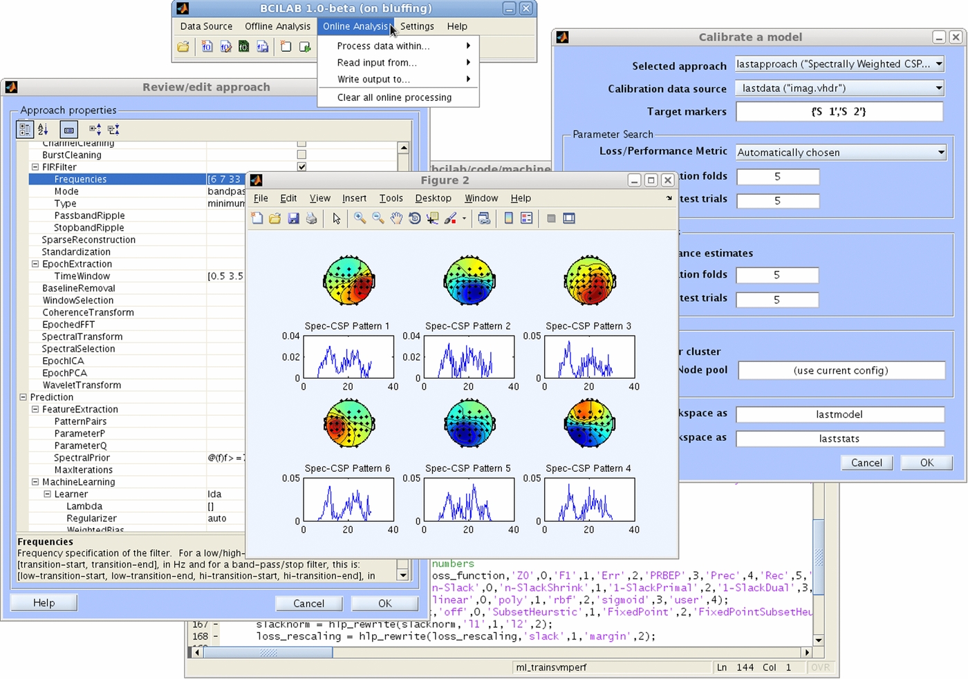
While technical capability is the primary driver of BCILAB, convenience for the user and developer is the second. This is reflected in a high level of (optional) automation, including automated artifact rejection, caching of intermediate results in memory and on disk, automatic GUI generation for all plug-ins, transparent (re-)compilation of MATLAB 'mex' binaries, and semi-automated build, unit testing, and cluster computing. As a result of this high level of automation, most scripts for offline or online processing can be written in 3–5 lines of MATLAB code (see appendix A for an example). Likewise, GUI-based design of new BCI approaches (see figure 1) can often be accomplished with only a few mouse clicks by employing the widespread supply of default parameters in BCILAB, automated parameter search commands, and so on. The flip-side of this high level of automation (as a conscious trade-off), is that it can at times be cumbersome to trace the control flow in hunting the source of an error.

**Figure 1.** Sample subset of BCILAB's GUI panels showing the main menu, a model visualization, a model configuration dialog (left), an evaluation setup dialog (right), and the script editor.
Download figure:
Standard image High-resolution image

2.8. Extensibility

The coding requirements for integrating of a new plug-in into the framework—a major concern for methods researchers—are kept relatively small. For most types of plug-ins, less than five lines of 'contract' code are required for seamless framework integration (see also appendix B). Many plug-ins thus comprise less than a page of MATLAB code each. Since the toolbox is open source, several well-documented plug-in examples are available.

2.9. Documentation

Comprehensive user and developer documentation is another focus of BCILAB. The documentation, available in the form of help files, plus a lecture series, an online wiki² and a developer tutorial, currently cover most individual methods relatively extensively (including full paper references and 200+ code examples). The code itself is documented to a high standard. Some areas of the documentation are nonetheless still under development, in particular descriptions of the implementation of novel paradigm plug-ins and top-down conceptual exposition of the relatively complex inner workings of the toolbox itself.

2.10. Summary

In summary, the design strengths of BCILAB are its focus on ready use of a large set of advanced/modern modeling methods, a forward-looking conceptual framework, adequate integration of neuroscientific knowledge, convenient and rapid prototyping, streamlined extension mechanisms, comprehensive automation, and sufficient documentation. Its lesser focus on native support for acquisition hardware and stimulus-presentation software is compensated for by built-in cooperativity with existing platforms specialized for real-time applications.

3. Architecture

3.1. Layered structure

The BCILAB toolbox is a collection of loosely coupled components organized in layers, any component depending only on elements in the layers below it (see figure 2).

**Figure 2.** BCILAB architecture diagram showing the four major layers and some most commonly used components.
Download figure:
Standard image High-resolution image

3.1.1. Dependency layer

The lowest layer is a collection of externally-maintained libraries (BCILAB's dependencies), such as machine learning packages and solvers including LIBSVM [36] and DAL [37], MATLAB toolboxes such as CVX [38] and BNT [39], and a GUI framework.

Canonical and compatibility-tested versions of the dependencies are included with permission in the BCILAB download and need not be obtained separately. With few exceptions, the dependency packages are unmodified and used through their official interfaces, so that manually updating them is often painless. In cases where modifications had to be made (such as bug fixes or compatibility changes) these are usually minimal and documented in the readme file accompanying the respective package. Dependencies are occasionally being updated with new BCILAB releases if there is compelling reason (such as major fixes or added features), although this is in practice rather rare—particularly for packages implementing specific published methods with fixed feature sets. A small fraction (5–10%) of the supported computational approaches use packages whose commercial use may require permission by the package author or is otherwise restricted—therefore commercial users should consult the readme files of the used packages. Academic/research and personal use is permitted in all cases. Some computational approaches currently depend on MATLAB's Signal Processing toolbox (although alternative techniques are included for the most frequently used methods) and some approaches and advanced framework features currently depend on the Statistics toolbox (such as some artifact removal functions). No other toolboxes are necessary, although some methods may optionally use other toolboxes, such as the Parallel Computing toolbox to leverage GPU computation.

3.1.2. Infrastructure layer

The second layer is the infrastructure including components for auto-generation of function GUIs, high performance (parallel/cluster) computation, disk caching of results, helper functions, and environment services (testing, deployment, etc).

3.1.3. Plug-in layer

A third layer is the included collection of user-supplied and built in plug-ins: here method developers may add new components. It is also the place where all BCI-specific functionality is located. Currently, four categories of plug-ins are recognized (most implemented as a single MATLAB function or two): Signal Processing plug-ins (digital filters and other signal processing algorithms), Machine Learning plug-ins (statistical learning and prediction functions), BCI Paradigm plug-ins organizing the processing stages (applying filters, feature extraction, and machine learning methods according to a particular template, sometimes also referred to as structural plug-ins or BCI templates), and Device plug-ins (adding support for input or output devices/protocols). Further details are given below.

3.1.4. Framework layer

Above the plug-in layer sits the framework layer, constituting the main internal 'clockwork' of BCILAB. This layer contains facilities to set up plug-ins, to execute them (either in real time or offline on pre-recorded data sets), for simulating and assessing their performance (including CV and pseudo-online analysis), and for visualizing BCI model parameters.

3.1.5. User-interface layer

The topmost level of the toolbox comprises the GUI and the scripting interface (the collection of scripting commands available in BCILAB), through which the user can interact with the rest of the toolbox.

3.2. Online processing

The most fundamental entity type maintained by BCILAB during online operation is the signal (a multi-channel time series, possibly segmented, with fixed but arbitrary sampling rate). This is represented as a backwards-compatible extension of the EEGLAB dataset structure (data plus arbitrary metadata) [40]. Signals represent recordings held in memory for offline processing, as well as brief chunks of data that are in flight during real-time processing. Most generally (although usually invisible to the user), processing is performed at the granularity of signal bundles, collections of one or more signals (of possibly different sensor types) that refer to overlapping or identical time periods (i.e. a recording). For example, these signals may include EEG, eye tracking, and/or motion-capture data from experiments using a mobile brain/body imaging (MoBI) approach [41].

Signals are transformed by signal processing plug-ins (called filters below for short), each of which is a function that takes one or more signals plus optional parameters and returns a processed version of that signal (also possibly adding or changing metadata). Some filters may have internal state, similar to MATLAB's built-in filter function, so as to perform time-varying processing on subsequent signal pieces. Multiple filters, their inter-connections, and their parameters are represented in a data structure called a filter graph (effectively a list of filter chains or trees).

While filters go a long way towards implementing an online BCI application, a complete BCI model in the toolbox is a two-part object, consisting of both a filter graph and a prediction function (see figure 3). The prediction function operates on the output of the filter graph (usually on a fixed-length time window over this output), can be invoked on demand at any time and latency, and returns a single result for the given data window (interpreted as a cognitive state estimate for the last time point in the window). For efficient processing, most paradigms return multiple estimates whenever data containing multiple segments/windows are passed to them. The internal steps performed by the prediction functions differ between BCI approaches—most current BCI designs perform a feature extraction step followed by a statistical mapping (typically using a machine learning method), while some perform a single joint mapping with no such distinction. BCILAB offers templates to aid the creation of both BCI types.

**Figure 3.** Online processing data flow in BCILAB for an example BCI model.
Download figure:
Standard image High-resolution image

To drive online processing computations, the toolbox offers a framework of functions for incremental data processing (independent of the actual wall-clock time) that may be supplied with streaming data from an acquisition device, pre-recorded data sets, signal generators, or from an enclosing experimentation environment such as BCI2000 or OpenViBE. The basic mechanisms offered by this online framework are declaration of the involved input streams (particularly their format) and processing pipeline (or predictive model) to use, appending a chunk of data to a stream, and querying the output of a processing pipeline (or predictive model) at the most recent sample of data appended so far. Consequently BCILAB's processing mechanisms can be driven by a hand-written fetch-process-output loop, for example integrated with the PsychToolbox, or by external processes calling into MATLAB such as BCI2000's bci_Process function, or by MATLAB timers to issue data fetching and processing in periodic intervals. Support for BCI2000 as external caller has already been implemented, while the equivalent support for OpenViBE still has to be added. Furthermore the toolbox provides a range of convenience plug-ins with GUIs to periodically ferry data into and out of the toolbox via timer-driven updates from various acquisition/output mechanisms (e.g., the lab streaming layer or TCP), which can also be run concurrently (within the limits of MATLAB's single interpreter thread). In addition to this continuous-processing fashion one may also query BCI predictors on demand based on custom application events, although such uses currently need to be scripted manually.

Online analysis is complemented by two primary offline processing pathways, namely model calibration and model evaluation, explained in the following, as well as several other tasks (including visualization, batch processing, and data curation) that will not be discussed at length in this paper.

3.3. The model calibration process

Model calibration, the most complex process in many modern BCI systems, is the process of integrating information from a variety of data sources and extracting from them an optimal set of parameters specifying a model that is custom-tailored to a particular person, electrode montage, and (often) situation or task. Individualizing BCI models is necessary because for any two persons, the optimal BCI models have different parameters (a consequence of person-to-person differences in brain geometry and functional organization, plus session-specific, montage-specific and task-specific effects).

Calibration is usually framed as one or a series of optimization and/or inference problems. Inference of such optimal parameters for a BCI model is a challenging and open research problem that shares many commonalities with diverse areas at the forefront of computational intelligence, data mining and machine learning. The primary source of data used to calibrate a BCI model is the calibration recording in which some knowledge about the changing cognitive and/or behavioral state of the subject is stored as annotations (usually instrumented during recording in the form of instructions or tasks given the participant to elicit specific cognitive states, behavior or behavioral intents while the data are being recorded). An important current research challenge is the adequate integration of information across multiple calibration sessions and/or subjects so as to form either a functional universal (non-person specific) model or a more accurately determined personalized model and yet another challenge is the principled integration of prior knowledge and constraints from neurophysiology [1].

In BCILAB, the computational processes of calibration and prediction are organized by the structural (paradigm) plug-ins. These plug-ins, which can be viewed as BCI design templates, are MATLAB objects with both a calibrate function (taking a collection of calibration data sets) and a predict function (taking a stream bundle). Internally, these tend to make use of some signal processing and machine learning plug-ins. In the most frequently used setting, calibration amounts to first filtering (i.e. pre-processing) the raw signals through a series of stages, followed by (possibly) adapting and extracting features for each trial, then finally training a classifier or regressor on the training data, all of which together make up the parameters of the resulting BCI model.

3.4. The model evaluation process

Model evaluation serves to assess the predictive performance (e.g., accuracy) of a BCI model, or more generally the performance of a particular computational approach (allowing determination of the best way to derive and apply such models under some given circumstances). Model evaluation amounts to applying a model to a data set for which changes in the subject's cognitive state or intent over time are known, then comparing the model's predictions with the known target values. A computational approach itself is evaluated by calibrating models according to this approach on some data sets ('training sets') and then testing the resulting models on separate testing sets—a process that can also be performed by sub-dividing a single set repeatedly into disjoint training and testing subsets, a process then called CV. This is usually done by invoking the same code used for online execution. The result of such an evaluation process is a 'loss' estimate, for example mis-classification rate (percentage of mis-classified data examples). Loss estimates can be used to statistically compare models or methods against each other. For this purpose BCILAB offers a variety of commonly used loss measures.

3.5. User interfaces

From a user's perspective, these operations are all performed through the top-level GUI or scripting interfaces, in particular the bci_train function to calibrate ('train') a model using a computational approach, the bci_predict function to apply a model offline on some recording with known ground truth markers, the bci_annotate function to generate a time course of a model's simulated outputs for some recording, and the bci_visualize function to display a model's internal parameters. Batch analysis is handled by the bci_batchtrain function. Further interfaces exist for real-time acquisition of streaming data (onl_newstream, onl_append, onl_read_background), and for loading and running BCI models on these data (onl_newpredictor, onl_predict, onl_write_background).

4. Analyzing experimental data

Practical data analysis using BCILAB is relatively straightforward and streamlined. The hardest part of the process is to bring the input data into a format that is accepted by the processing pipeline, and to configure the pipeline as desired (in particular for heavily customized analysis approaches), while the coding effort is typically very low to zero. In this section, two representative experimental tasks are introduced and an analysis process outlined for each of them. For reasons of scope we restrict ourselves here to two BCI problems that are reasonably well understood and cover two types of underlying neurophysiological processes (oscillatory and slow-wave) that are particularly relevant for current BCI systems. We consider the first one in the context of directly controlled active BCIs and the second one in the context of passive cognitive state assessment (see also [13] for definitions). Since it is not possible to cover more than a small fraction of relevant uses in the scope of this paper some more advanced analysis problems will be treated in a subsequent article.

4.1. Imagined movements task

Task A is a variant of the well-established motor imagery task in which a subject is given a sequence of on-screen instructions to imagine one of several different motor activities (e.g., to imagine moving the left hand versus the right hand), repeated over a few dozen trials in a ∼15 to 60 min session [42]. This has traditionally been one of the two most frequently used experimental designs in the clinical BCI field (the other being so-called P300 spelling [43, 44]), and is a widely accepted benchmark. For reasons of reproducibility, we use here three publicly available data sets from BCI competitions III and IV, which together comprise data from 17 subjects. For comparability our analysis of this task largely replicates that of [45] up to minor differences in analysis parameters.

4.1.1. Data

The first collection of recordings (here denoted as A.1) is available as dataset IVa³ of the BCI competition III, recorded at the Berlin Institute of Technology [46]. This comprises data from five subjects (designated aa, al, av, aw, ay) who imagined right hand versus foot movements while 118 channels of EEG were recorded at 100 Hz. Of a total of 280 recorded trials, the first 168/224/84/56/28 trials for the respective subject were used for training; remaining trials were used for testing.

Dataset A.2 is the dataset IIIa⁴ of the BCI competition III, recorded at Graz University [47]. It comprises data from three subjects (k3, k6 and l1) who performed 45/30/30 trials imaging movement of left hand, right hand, feet, or tongue during recording from 60 EEG electrodes at 250 Hz. We considered here only trials imagining left-hand versus right-hand movements and ignore the other trials. Note: the trials available for testing in A.2 were interleaved with the training data, likely producing somewhat optimistic results (see also [25]).

Dataset A.3 was published as data set IIa⁵ of the BCI competition IV, also from Graz University, comprising data from nine subjects who performed 72 trials each, imagining left hand, right hand, feet, and tongue movements [48]; here we also restrict ourselves to left versus right hand movements. EEG was recorded from 22 channels at 250 Hz.

The experiment designs for A.1 and A.3 are nearly identical and are structured as follows. Each trial begins with presentation of a fixation cross on a black background accompanied by a beep. After 2 s, an arrow-shaped cue pointing either left, right, up, or down is presented to indicate the type of movement to imagine, and remains on screen for 1.25 s. Subjects were asked to carry out the cued imagination task until the fixation cross disappeared from the screen (6 s after the beginning of the trial), followed by a short break with a black screen. This design was chosen to simulate a paralyzed (locked-in) patient communicating by imagining movements, for example to control a cursor on screen (although here performed by healthy subjects). A.2 was a simplified variant of the task with different timing. In each case, the goal of the BCI analysis is to accurately estimate the type of movement imagined in each trial based on the recorded EEG data.

4.2. Rapid serial visual presentation task

Task B is an example of a non-clinical cognitive state assessment problem that was chosen to illustrate the use of BCI methods that operate on event-related potentials (ERPs). The task is a variant of the rapid serial visual presentation (RSVP) task as reported in [49] in which the subject is presented an RSVP sequence of satellite images (at 12/s), one of which may contain a target object—here an airplane. This experiment simulated a human brain response-aided search through a large volume of satellite data. Here images were presented in 4.1-s bursts, after each of which the subject is asked to indicate whether the burst contained a target image or not. Each burst was preceded by a 1 s fixation cross and contained either zero (40%) or one (60%) target image. The total number of target images per session was 290, while the number of non-target images was 24 104. The goal of the BCI analysis here is to correctly estimate whether an image presented during the burst contains a target object or not based on the user's EEG immediately following each image presentation. EEG used in the analysis was collected from 128 scalp sites at 256 Hz.

4.3. Analysis methods

The two tasks elicit the two major EEG phenomena used in BCI approaches today, namely (in task A) modulations of the power spectra of oscillatory processes [50], in particular cortical idling rhythms, and (in task B) regularities in slow cortical potentials, often measured using event-locked trial averages as ERPs [51].

4.3.1. Methods for oscillatory processes

For oscillatory processes, in task A inducing so-called event-related synchronization and desynchronization [52] phenomena, a variety of methods have been developed and their relative merits are in many cases well established. Our analysis therefore aims at demonstrating expected results on well-understood data using BCILAB. We compare three families of methods. First, we illustrate the use of logarithmic bandpower estimates (log-BP) often used in the early days of BCI design [53, 54], in particular a method operating on three standard electrode channel placements over motor cortex (C3,Cz,C4) called here BP-MC, plus a variant operating on all channels called BP-AC.

The second method family includes variants of the highly popular common spatial patterns (CSP) algorithm [55]. We compare the basic CSP algorithm with three of its more recently proposed regularized forms (see [45]). Two of these adaptively shrink the underlying covariance-matrix estimates towards a diagonal matrix (also known as diagonal loading CSP or DLCSP) using either cross-validation (DLCSPcv) or analytical shrinkage (DLCSPauto) as in [56], while the third penalizes the spatial filters in an approach called Tikhonov-regularized CSP (TRCSP) [45].

While these CSP variants operate on a single frequency band (usually a 'wideband' 7–30 Hz window for motor imagery task data), the implemented variant of the filter-bank CSP approach (FBCSP) [57] instead solves one CSP instance per frequency band of interest and pools the resulting features. The last member of the CSP family compared here, spectrally weighted CSP (Spec-CSP) [22], adaptively learns relevant spatial and spectral weights using an alternating update procedure. Spec-CSP has been shown [22] to be roughly comparable in performance to other adaptive state-of-the-art frequency-learning methods such as CSSP [58] and CSSSP [59], which are therefore not discussed here.

The third family of methods compared here might be called single-stage methods because they do not split the learning into a separate feature-extraction and classification stage, but rather solve these problems jointly as a single (here convex) optimization or learning problem, the main appeal being the guarantee of meaningful global optimality. The representative chosen here, a trace-norm regularized logistic regression on a second-order representation of the signal, has been shown to be one of the best-performing members of this class [60]. We include two variants of this method, one applied to the wideband window (DALwb, where DAL stands for the dual-augmented Lagrangian, the name of the optimization framework) and a variant applied to multiple bands (8–13 Hz, 15–25 Hz and 7–30 Hz, here called DALmb). For most methods the underlying band-pass filtering has been performed using a minimum-phase causal FIR filter (7–30 Hz, actual transition bands 6–8 Hz and 28–32 Hz), except for Spec-CSP and the multi-band approaches, where FFT-based spectral reweighting was used. In all data sets, the time window over which the oscillatory features (e.g., signal variance) were computed was 0.5 s to 2.5 s following the cue stimulus.

4.3.2. Methods for slow cortical potentials

For slow cortical potentials and ERP-based modeling, one of the most frequently used methods is what we call here the windowed means approach, a linear model, typically linear discriminant analysis (LDA) [61], applied to per-channel averages of the EEG signal over one or more short time window segments, possibly with additional preprocessing (see [62] for a good tutorial). In this approach, the classifier typically operates on multi-channel segment averages of the raw (or band-pass filtered) signal and implicitly applies linear spatial filtering (if the classifier is linear) to best recover the event-related signals of the underlying neural generators while minimizing other EEG source activities (brain or non-brain) that also contribute to the channel EEG signals through linear electromagnetic volume conduction.

However, since the number of features (channels by time windows) is typically high compared to the number of trials, a variety of methods have been introduced in the literature to better constrain the admissible solutions and ameliorate over-fitting of the model to spurious patterns in the training data (part of 'the curse of dimensionality'). This is often done as part of the classifier definition, for example by using the more robust shrinkage LDA [56] or logistic regression with either an l2 regularizer or Gaussian Bayesian prior [63]. Use of a shrinkage LDA variant and Bayesian logistic regression are illustrated here under the names WM-LDA and WM-LR.

The other approach to dealing with over-fitting operates at the level of the underlying features, for example finding a more parsimonious set of time windows or operating on a wavelet representation of the channel data (leading to a better concentration of relevant information into a few features, thus allowing the use of sparse classifiers). We include an approach (here named WL-GS) that operates on wavelet features using a regularized logistic regression classifier with group-sparse (L1/L2) regularization, where each group is represented by the activations of a given wavelet basis function across channels. This is an example of a custom approach that is however easy to design using built-in BCILAB tools.

A third approach illustrates the use of machine learning methods that rely on domain-specific structural assumptions (in the form of custom regularization terms) that are believed to be appropriate for the underlying EEG data. One such approach is the recently-introduced first-order dual-augmented Lagrangian method with dual-spectral regularization [60], here included as DALERP. Lastly, we compare a logistic regression (here named Raw-GS) that (like DALERP) also operates on the raw channel data, but is group-sparse in features grouped by samples (using a similar assumption as in WL-GS).

4.4. Analysis procedure

4.4.1. Evaluation strategy

While the most realistic measure of BCI performance is user performance in a particular BCI-assisted task (e.g., information transfer rate in a spelling task or user efficiency in a BCI-assisted operator scenario), such measures do not lend themselves well to comparison of results from different methods on the same data. Therefore, in practice performance is often measured using offline prediction accuracy and/or related measures, either on a separate labeled test set (when such data are available), or using CV (when only a single recording per subject is available). While a great number of reported BCI results have been obtained using randomized CV (an established standard in the machine learning community), a less (overly) optimistic measure is block-wise (a.k.a., chronological) CV. Ideally, such procedures should leave unused data margins between the training and test sets to avoid intermingling of their data features through local-in-time correlations. Results for the latter approach (five-fold block-wise CV with five-trial margins) are reported here for task B and compared to performance on a separate test set. The performance of the classifiers on task A is measured by mis-classification rate, and on task B by area under the receiver operator curve (AUC) since in this task there are many more non-target than target stimuli.

For approaches that contain free parameters that need to be optimized (most importantly, regularization parameters), a CV guided grid search is employed within the respective training sets. This is known as nested CV (here 5×5).

4.4.2. Analysis process

Data from both tasks were analyzed using the batch analysis facility of BCILAB (the complete scripts are available at a supplementary webpage⁶). In each case separate training and test data sets were available. Nested CV was performed within each training set, and the resulting model was applied to the test set. For task A, a representative excerpt of the batch analysis script is given in figure 5. This analysis script reproduces the results for the CSP, Spec-CSP, TRCSP and DALwb approaches. For task B, a screen shot of the GUI configuration dialog for one of the methods (DALERP) in shown in figure 4.

**Figure 4.** Core settings in the BCILAB dialog window for the DALERP paradigm. The highlighted text is the time window parameter as customized for task B (epochs: −0.2 s to 0.8 s relative to stimulus presentation). This dialog is auto-generated from the parameter descriptions of multiple BCILAB plug-ins used by DALERP. Each approach also has an extended settings dialog window; an example is shown in figure 1, left.
Download figure:
Standard image High-resolution image

5. Analysis results

5.1. Classification performance for task A

For the task A data, the classification accuracies of all algorithms across data from all subjects are summarized in table 2. Chance level here is 50%. In particular, it can be seen that the relatively simple channel band-power classifier forms the low anchor at median 59.0% performance, followed by the same approach restricted to a few key channels (C3, Cz, and C4). Filter-bank CSP is in the same performance regime at 66.5%, possibly because of overfitting or degradation of the LDA applied to relatively few training trials at high dimensions (as in data set A.1).

Table 2. Classification accuracies of the compared approaches for each subject's data in task A.

	aa	al	av	aw	ay	k3	k6	l1	1	2	3	4	5	6	7	8	9	Median	Mean/std
BP-MC	58.0	82.1	62.2	72.3	72.6	88.9	45.0	75.0	54.9	52.1	54.2	59.0	52.8	45.8	56.3	61.1	79.9	59.0	63.0 ± 13.0
BP-AC	59.8	92.9	64.3	60.3	73.8	76.7	51.7	70.0	58.3	50.7	77.1	57.6	61.1	55.6	53.5	65.3	77.1	61.1	65.0 ± 11.4
CSP	68.8	96.4	74.5	80.4	75.8	96.7	58.3	96.7	82.6	48.6	89.6	69.4	60.4	61.1	56.9	89.6	82.6	75.8	75.8 ± 15.3
TRCSP	68.8	96.4	73.5	80.4	75.8	94.4	58.3	96.7	84.7	50.0	88.9	66.7	58.3	61.8	53.5	88.2	82.6	75.8	75.2 ± 15.4
DLCSPcv	69.6	96.4	71.9	80.4	76.2	94.4	58.3	96.7	82.6	50.0	93.1	68.1	57.6	59.0	52.1	90.3	84.0	76.2	75.3 ± 16.0
DLCSPau	67.9	96.4	72.4	85.3	78.2	95.6	60.0	96.7	83.3	47.2	90.3	68.1	56.9	61.1	53.5	90.3	87.5	78.2	75.9 ± 16.3
SpecCSP	75.0	98.2	71.4	77.7	77.4	96.7	43.3	96.7	80.6	53.5	94.4	60.4	57.6	61.8	59.0	89.6	87.5	77.4	75.3 ± 17.1
DALwb	75.0	96.4	71.4	81.7	48.0	93.3	56.7	98.3	81.3	49.3	91.0	70.1	59.7	63.9	49.3	88.2	81.9	75.0	73.9 ± 17.1
DALmb	75.0	96.4	72.4	81.7	48.0	90.0	70.0	98.3	84.0	51.4	91.0	66.0	59.0	62.5	64.6	90.3	88.2	75.0	75.8 ± 15.7
FBCSP	66.1	96.4	66.3	66.5	48.4	97.8	70.0	90.0	82.6	51.4	88.9	63.2	63.2	58.3	61.1	89.6	89.6	66.5	73.5 ± 16.0

Remarkably, both the Spec-CSP (model parameters shown in figure 5) and DAL approaches perform only marginally better, despite having been shown to be superior to CSP on large data corpora [22]. This effect might be attributed to the competition data sets used here often being deliberately of less-than-optimal quality or being otherwise challenging for standard methods. Almost 10% better than the bandpower approaches is common spatial patterns, which uses analytically derived spatial filters. The second-order dual-augmented Lagrangian approach, using alpha (8–13), beta (15–25) and mu (7–30) frequency bands, gives about the same performance (with no significant difference under a standard paired t-test). In agreement with the literature [45], the highest accuracy across all the data is attained by the three regularized CSP algorithms TRCSP, DLCSPcv and the recently-proposed DLCSPauto.

5.2. Classification performance for task B

Applied to task B data, in cross-validated performance on the training set the two group-sparse approaches WL-GS and Raw-GS significantly out-performed the windowed means approaches WM-LDA and WM-LR (p < 0.01 in a paired t-test). This difference can in part be explained by the (not necessarily optimal) ad hoc dimensionality reduction that is typically imposed by pre-selecting windows of interest for windowed means approaches to operate on. On the separate test set, the two group-sparse WL-GS and Raw-GS approaches significantly out-performed the windowed means approaches (p < 0.05 in a paired t-test). The full listing of results is given in table 3. The DALERP approach, for which the model parameters are shown in figure 6, gave mean accuracies between these low and high anchor points that were not significantly different from other approaches—either on the training set or the test set. The inability of the DALERP approach to out-perform any other method might be explained by the fact that DALERP encourages weight matrices corresponding to spatial filters that stay constant over the course of the entire epoch, in contrast to the other methods involving time-varying spatial filters that can more successfully focus on evolving or propagating active source constellations.

**Figure 6.** The two most highly-weighted DALERP components (spatial filters and weight time courses) for subject 1 data in task B (AUC = 0.88). Five more components were learned for this subject (not shown). Components similar to these two were learned by DALERP for most of the subjects.
Download figure:
Standard image High-resolution image

Table 3. Test-set performance (area under curve) for each subject in task B, including mean and standard deviation. The last two columns show the performance as estimated via five-fold CV on the training set (mean and std dev.).

	s1	s2	s3	s4	s5	s6	Mean	Std	CV mean	CV std
WM-LDA	0.85	0.48	0.80	0.57	0.58	0.71	0.66	0.14	0.87	0.07
WM-LR	0.85	0.53	0.81	0.59	0.52	0.90	0.70	0.17	0.88	0.08
DALERP	0.88	0.52	0.74	0.74	0.55	0.93	0.72	0.17	0.88	0.06
WL-GS	0.87	0.58	0.84	0.64	0.63	0.94	0.75	0.15	0.91	0.06
Raw-GS	0.86	0.55	0.81	0.64	0.60	0.94	0.73	0.16	0.91	0.07

6. Discussion

The results of the presented methods comparisons show that state-of-the-art BCI performance can be readily achieved by applying BCILAB to representative BCI task EEG data, using either features adapted to oscillatory processes or to event-related slow-wave scalp potentials. Using the relative flexibility and versatility of the BCILAB framework we could implement, apply and compare a considerable number of representative methods, among them some state-of-the-art approaches including the group-sparse wavelet approach to ERP detection and the DALERP approach. Once the required building blocks are in place, constructing BCI approaches either using the GUI (as for task B) or the scripting interfaces (as for task A) is a straightforward and efficient process, amounting to composing only a few lines of script code, and producing publication-ready method and data set comparison results. Task B illustrates the applicability of BCI methods and tools provided by BCILAB to questions of interest in the field of human–computer interaction, such as whether a particular visual event was perceived by the interface user. While this is a simple example, the general principle of using BCI measures to augment human–computer interaction has already been applied in a wide variety of scenarios (e.g., workload estimation [64, 65], passive attention deployment [66], error responses [67–69], and drowsiness monitoring [70]).

Implementations of all methods for which offline results were provided here are included with the toolbox in form of tutorial scripts that have been tested offline, pseudo-online (that is, with incremental processing), and in real time on a variety of machines and on tutorial data sets included with the toolbox download package. Statistics for method comparisons (for example, t-tests) are not yet part of the BCILAB toolbox but can be computed relatively easily either through native MATLAB tools or by exporting the results to a statistics package.

7. Conclusion

We have introduced a new toolbox for BCI design that offers tools for efficient brain data analysis, both for experimental scientists and for methods developers. BCILAB also offers streamlined extension mechanisms both for incorporating new building blocks and for connecting to external applications and acquisition hardware. We have provided empirical evidence that the framework and some key algorithms are implemented in accord with the respective literature and give the expected results on well-known BCI competition data. We view the open-source software release accompanying this paper as the starting point of a long-term interactive community process in which the scope and scale of BCILAB may well far outgrow the present software package. Our hope is that use of BCILAB will accelerate research on advanced BCI methods and thereby shorten the time required to develop a well-founded and reasonably complete theoretical and empirical basis for real-time analysis of brain signals for a wide range of purposes.

Acknowledgments

The BCILAB toolbox was primarily developed by CK at the Swartz Center for Computational Neuroscience, UCSD with contributions from T Mullen, C Brunner and L Frolich and supervision by SM. Development of this software was supported by the Army Research Laboratories under Cooperative Agreement Number W911NF-10-2-0022, as well as by a gift to UCSD from the Swartz Foundation (Oldfield, NY). The views and the conclusions contained in this document are those of the authors and should not be interpreted as representing the official policies, either expressed or implied, of the Army Research Laboratory or the U.S Government. The U.S Government is authorized to reproduce and distribute reprints for Government purposes notwithstanding any copyright notation herein. BCILAB builds on other open-source tools, including EEGLAB [40] and various machine learning and signal processing toolkits. The architecture was inspired by an earlier toolbox (The PhyPA Toolbox) developed by CK with contributions from T Zander at the Center for Human-Machine Systems, TU Berlin. We thank the anonymous reviewers for their very useful feedback and constructive comments.

Appendix A.: Batch analysis script for data of task A

The following code listing is a shortened yet fully functional excerpt of the BCILAB analysis script used to reproduce the performance results listed in table 2 (task A) for the methods CSP, Spec-CSP, TRCSP and DALmb.

Appendix B.: Example signal processing plug-in

The following MATLAB function is an example of a basic filter plug-in that processes epoched signals; placing a function like this in the code/filters directory of the toolbox will lead to its automatic detection and inclusion in the available analysis pipelines and GUIs. The mandatory framework contract consists of the exp_beginfun and exp_endfun prologue/epilogue lines (as well as the calling convention of the input signal being either the first positional argument or the name-value pair with name 'Signal'). The declare_properties and arg_define clauses are optional but enable seamless integration into the default filter chain and the GUI, respectively. The bold section is the actual signal processing code.