Spatiotemporal Change of Eco-Environmental Quality in the Oasis City and Its Correlation with Urbanization Based on RSEI: A Case Study of Urumqi, China

Abstract

As an important node city of “The Belt and Road” strategy, Urumqi has a non-negligible impact on the ecological environment in the process of rapid development. It is of great significance to understand the coupling and coordination between urbanization and the ecological environment for regional sustainable development. However, previous studies on the coupling coordination degree (CCD) model of urbanization and ecological environment are limited, and they ignore the endogenous relationship between the two. Therefore, this study aims to introduce an econometric model, the panel vector autoregression model (PVAR), to further explore the relationship between them and the influencing mechanism. Firstly, urbanization and ecological environment were evaluated objectively by the comprehensive nighttime light index (CNLI) and remote sensing ecological index (RSEI), respectively. Then, the coupling coordination degree of urbanization and the ecological environment were evaluated comprehensively by a typical coupling coordination degree model. Finally, the PVAR model is used to analyze the interaction between the two systems and the mechanism of action. The results showed that: (1) in the recent 25 years, the mean value of RSEI in Urumqi decreased gradually, and the overall ecological environment deteriorated, but the differences among districts and counties were still significant; (2) the urbanization level of Urumqi is on the rise, while UC, DBC(B), and MD have the highest increase in CNLI although they are at a low level; and (3) in the interactive relationship between urbanization and the ecological environment, the development of Urumqi’s ecological environment is mainly affected by its development inertia, and the development of urbanization is limited by the ecological environment. This study fills the gap in the study of the interaction mechanism between urbanization and the ecological environment and provides a new perspective for the study of sustainable urban development worldwide.

1. Introduction

Urbanization is one of the most important human activities on Earth since the Anthropocene [1]. In this era of globalization, the world is urbanizing rapidly. According to UN-Habitat, at the beginning of the 21st century, about 50% of the world’s population lived in cities, and it is expected that by 2050, they will account for 70% of the total population [2]. It is worth noting that with the rapid development of urbanization, the regional ecological environment has undergone tremendous changes [3].

Over the past 30 years, China has been the fastest growing country in urbanization. China has experienced an unprecedented process of urbanization, with the urbanization rate rising from 26.41% in 1990 to 63.89% in 2020 (http://www.stats.gov.cn/, accessed on 14 April 2022). With the acceleration of urbanization, human activities (heat island effect [4], air pollution [5]) have increasingly interfered with the natural ecosystem, leading to a series of ecological environmental problems, such as land degradation [6,7], a sharp drop in ecological diversity [8], water shortage [9], etc. Meanwhile, in turn, the deterioration of the ecological environment will restrict urbanization and sustainable development [10]. Coordination between urbanization and ecological environment quality is the key to achieving sustainable development.

The unsustainability of rapid urbanization has inspired scholars to study the interaction between urbanization and the ecological environment [11]. For the study of the relationship between urbanization and eco-environment quality, Grossman et al. [12] put forward the theoretical relationship model of the “Environmental Kuznets curve” as early as in the 1990s, and then put forward the decoupling theory [13], urban metabolism theory [14], and coupling coordination degree model [15]. Compared with other methods, the coupling coordination degree model focuses more on describing the interaction between two or more subsystems [16]. Among them, Feng et al. [16] constructed a coupling coordination degree model based on statistical data, revealing a comprehensive framework for the interaction between urbanization and the ecological environment in the Pan-Third Pole region, and further explained the coupling mechanism of the two. Fu et al. [17] revealed the dynamic trend of urbanization and Eco-Environment development by establishing a comprehensive indicator system and applying it to the coupling coordination degree model. Based on statistical data, Guo et al. [18] constructed a coupling coordination degree model from multiple dimensions and conducted a coupling analysis of urbanization and ecological environment quality in Liaoning Province. In terms of research data, the above data are mostly based on panel statistics but lack spatial information. The above studies only studied the coupling coordination between systems, resulting in an unclear coupling mechanism between the ecological environment and urbanization.

With the continuous development of remote sensing technology, remote sensing nighttime light has been proved to be highly correlated with social economies, such as population [19] and economic activities [20,21]. Considering the respective advantages of daytime optical remote sensing and nighttime light remote sensing in revealing the status of the ecological environment and characteristics of urbanization, scholars began to try to integrate the two types of remote sensing data to carry out the coupling study of urbanization and ecological environment [22]. For example, Anees et al. [23] explored the relationship between vegetation cover (FVC) and human activities in Pakistan using nighttime light data. Lemoine-Rodríguez et al. [24] explored the relationship between land reflected temperature (LST) and urban form in cities located in different climates based on nighttime light data. Liu et al. [25] used nighttime light data and NDVI to characterize the spatiotemporal relationship between urbanization and vegetation degradation in different metropolises around the world. However, most of the above analysis was based on a single ecological index, which could not reflect the comprehensive ecological status of the study area.

Compared with the traditional ecological evaluation of a single remote sensing index, in 2013, Xu [26] obtained several factors that could directly reflect ecological conditions through Remote Sensing information inversion and constructed a new ecological evaluation index—‘Remote Sensing based Ecological Index’ (RSEI) based on Remote Sensing data, which coupled several ecological indicators. RSEI is widely used in regional eco-environmental quality monitoring due to its diversity of indicators, the objectivity of weights, and the visibility of results. For example, Boori et al. [27] constructed RSEI based on Landsat satellite data to quantitatively analyze the ecological vulnerability of Samara, Russia. Alwan et al. [28] used RSEI to monitor and assess ecological changes in swampy southern Iraq over years. Taking central Iran as an example, Saleh et al. [29] constructed RSEI based on Landsat TM/OLI satellite data and assessed the ecological quality of Iran for 15 years. An et al. [30] compiled RSEI by using Modis data at the county level and investigated the ecological environment of the Three Gorges Eco-economic Corridor, further expanding the application scenarios of RSEI.

The implementation of the western development strategy and urbanization strategy, together with the further implementation of a new round of “aiding Xinjiang”, has had a positive impact on the leap-forward development of Xinjiang’s economy. In the context of rapid urbanization, Urumqi, the capital of Xinjiang, has experienced rapid economic development. Urumqi is a typical arid area with a fragile ecological environment. With the continuous growth of population and the continuous expansion of construction land, the regional ecological environment is facing increasingly severe pressure. How to protect the ecological environment and realize the coordinated development of economy and ecology in the process of urbanization has become an important problem faced by Urumqi. In this context, taking Urumqi as the research object, the comprehensive nighttime light index (CNLI) and the RSEI were used to objectively evaluate the urbanization and ecological environment. Then, a typical coupling coordination degree model is used to comprehensively evaluate the coupling coordination degree between urbanization and the ecological environment. Finally, the panel vector autoregression (PVAR) model was used to analyze the interaction and mechanism between the two systems. The research not only fills the gap in the research on the coupling mechanism of ecological environment quality and urbanization; but also provides a theoretical basis for land management and ecological protection in the context of rapid urbanization. The research flow chart is shown in Figure 1.

2. Study Area and Data sources

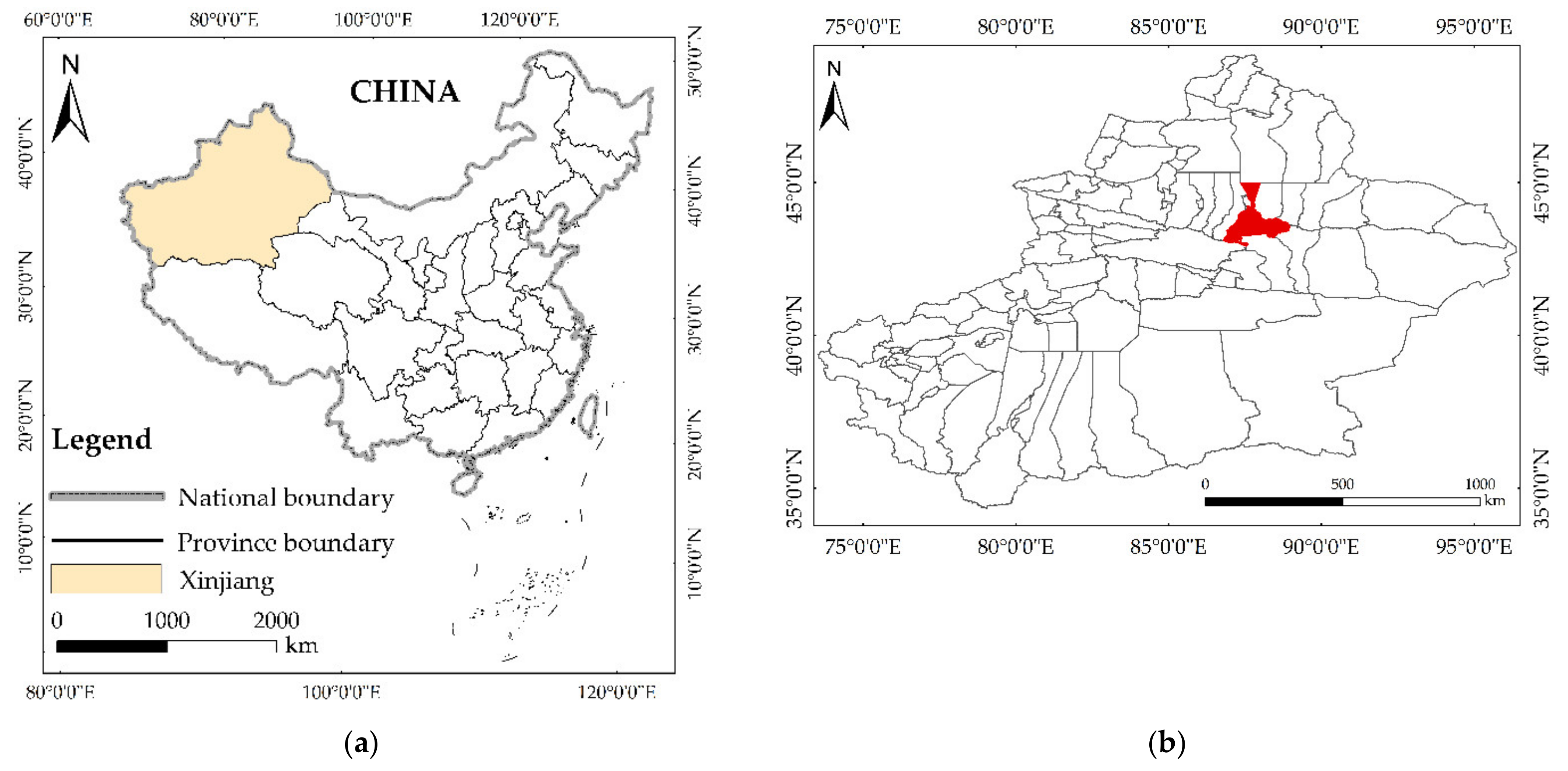
2.1. Study Area

Urumqi is located in the hinterland of Eurasia, at the northern foot of the middle Tianshan Mountains, and at the southern margin of the Junggar Basin (42°45′–44°08′ N, 86°37′–88°58′ E, as shown in Figure 2a). It has a temperate continental semi-arid climate with long sunshine duration, drought, little rainfall throughout the year, sparse vegetation, and a fragile ecological environment [31]; the land cover types in the study area are mostly deserts (Figure 2b). Urumqi is the capital of the Xinjiang Uygur Autonomous Region, the center of the Tianshan North Slope Economic Belt, and one of the core areas of the Silk Road Economic Belt. At present, Urumqi has a total area of 13,800 square kilometers, of which the urban area is 365.88 square kilometers, and the permanent population is about 4.0544 million, accounting for 15.68% of the total population of Xinjiang. Urumqi has seven municipal districts and one county, namely Tianshan (TS), Shayibake (SYBK), New Urban (NU), Shuimogou (SMG), Toutunhe (TTH), Dabancheng (DBC)), Midong (MD), and Urumqi County (UC). Geographically, UC is located in the middle of DBC (Figure 2). Therefore, this paper artificially divides DBC into DBC(B) and DBC(S). Urumqi’s development is unbalanced. The urbanization rate of Urumqi in 2020 will reach 94.52%, which is higher than the average urbanization rate of Xinjiang (56.53%). However, the urbanization rate of UC is only 20.75%. The above information comes from Urumqi Municipal People’s Government (http://urumqi.gov.cn, accessed on 14 July 2022) and ‘Xinjiang Statistical Yearbook 2020’.

2.2. Data Sources and Pre-Processing

The construction of the RSEI index requires four component index data, namely, greenness (NDVI), dryness (normalized difference impervious surface index, NDBSI), wetness (WET), and heat (land surface temperature, LST) components [26]. Therefore, based on these four components, this paper selects the corresponding standard products from the Landsat product database as data sources. Remote sensing image data from the U.S. Geological Survey (United States Geological Survey, the USGS) released by the Landsat data (https://earthexplorer.usgs.gov/, accessed on 16 April 2022), the spatial resolution of 30 m, the earth observation revisit period is 16 days. The TM Surface Reflectance data of Landsat 5 satellites from 1995 to 2010 and OLI of Landsat 8 satellites from 2015 to 2020 are accessed online through JavaScript API on the GEE platform Surface Reflectance data; geometric correction, radiometric correction, and atmospheric correction have been performed on the data (https://developers.google.com/earth-engine/datasets/catalog/landsat, accessed on 16 April 2022).

The image time thresholds of 1995, 2005, 2010, 2015, and 2020 (growth period: from June to September) are screened on the GEE platform, and the cloud pixels are removed from the input image data set that conform to the time and space range by using the officially provided Landsat cloud mask algorithm. The minimum cloud amount image of the target year in summer was synthesized from the median cloud-free pixel.

Night light remote sensing data can effectively record the radiation signals generated by artificial light in human activities. These data have been widely used to monitor and evaluate the development and change of multi-scale socio-economic activities [32,33,34]. Among them, the emergence of nighttime weak light detection sensors represented by OLS and VIIRS provides a new key method for the study of human activity intensity [22]. The nighttime light remote sensing dataset is obtained from published by Wu et al. [35] on the Harvard Dataverse platform. This dataset has been calibrated with DMSP-OLS data using the “pseudo-invariant pixel” method [36,37], and further improved to obtain DMSP-OLS (1992–2020) with a spatial resolution of 1000 m. This paper selects 1995, 2005, 2010, 2015, and 2020 nightlight data for resampling and projection.

The vector data include administrative division boundaries of Urumqi, and the data come from the “Resource and Environment Science and Data Center” (https://www.resdc.cn/, accessed on 16 April 2022). The detailed descriptions are shown in

Table 1. The detailed descriptions of the study data.

Data	Spatial Resolution	Time Resolution	Source	Function
Landsat 5, 8	30 m	16-Day	Google Earth Engine	Calculate the NDVI, NDBSI, WET, LST
DMSP-OLS	1000 m	Annual	Dataset ([35])	Calculate the LAP, MLI, CNLI
The administrative division data	1:1 million	2015	RESDC 1	Use basic base map data and perform zonal statistics

¹ Resource and Environment Science and Data Center.

.

3. Methods

3.1. Construction of Remote Sensing-Based Ecological Index (RSEI)

Select four components (Wetness, Greenness, Heat, and Dryness) that are closely related to the quality of the ecological environment to construct RSEI:

$$RSEI=f(Wetness,Greenness,Heat,Dryness)$$

(1)

The calculation formula of each ecological index is as follows:

(1)

Wetness: The wetness in RSEI is calculated by the wetness component wet in the tassel cap transformation [38], and the formula is as follows:

$$WE{T}_{TM}=0.0315{\rho }_{Blue}+0.2021{\rho }_{Green}+0.3102{\rho }_{\mathrm{Re}d}+0.1594{\rho }_{NIR}-0.6806{\rho }_{SWIR1}-0.6109{\rho }_{SWIR2}$$

(2)

$$WE{T}_{OLI}=0.1511{\rho }_{Blue}+0.1972{\rho }_{Green}+0.3283{\rho }_{\mathrm{Re}d}+0.3407{\rho }_{NIR}-0.7117{\rho }_{SWIR1}-0.4559{\rho }_{SWIR2}$$

(3)

where ρ_Blue, ρ_Green, ρ_Red, ρ_NIR, ρ_SWIR1, and ρ_SWIR2 represent the reflectance of ground objects corresponding to the TM image and OLI image in the Blue wave band, Green wave band, Red wave band, Near Infrared band, Short Wave Infrared 1 band, and Short Wave Infrared 2 band, respectively.

(2)

Greenness: The greenness of RSEI can be solved by the normalized difference vegetation index (NDVI) [25].

$$NDVI=\frac{{\rho }_{NIR}-{\rho }_{\mathrm{Re}d}}{{\rho }_{NIR}+{\rho }_{\mathrm{Re}d}}$$

(4)

(3)

Heat: The heat index of land surface temperature (LST) is obtained by a single window algorithm.

$$LST=T/[1+(\lambda T/\theta )\hspace{0.33em}·\hspace{0.33em}\ln \epsilon ]-273.15$$

(5)

where T: the luminance temperature of heat radiation intensity transformation; λ: central wavelength of the thermal infrared band; θ: constant, ε: surface emissivity. Please refer to the reference for the calculation method [39].

(4)

Dryness: the increase of building land and the impervious surface will cause the surface “dryness”. The Index-based Built-up Index (IBI) [40] and Soil Index (SI) [41] are selected to synthesize the dryness index.

$$NDBSI=\frac{SI+IBI}{2}$$

(6)

$$IBI=\frac{2{\rho }_{SWIR1}/({\rho }_{SWIR1}+{\rho }_{NIR})-[{\rho }_{NIR}/({\rho }_{NIR}+{\rho }_{\mathrm{Re}d})+{\rho }_{Green}/({\rho }_{Green}+{\rho }_{SWIR1})]}{2{\rho }_{SWIR1}/({\rho }_{SWIR1}+{\rho }_{NIR})+[{\rho }_{NIR}/({\rho }_{NIR}+{\rho }_{\mathrm{Re}d})+{\rho }_{Green}/({\rho }_{Green}+{\rho }_{SWIR1})]}$$

(7)

$$SI=\frac{({\rho }_{SWIR1}+{\rho }_{\mathrm{Re}d})-({\rho }_{Blue}+{\rho }_{NIR})}{({\rho }_{SWIR1}+{\rho }_{\mathrm{Re}d})+({\rho }_{Blue}+{\rho }_{NIR})}$$

(8)

Since the dimensions of the above four components are not uniform, standardization is required, and then principal component analysis (PCA) is performed. Principal component analysis can effectively recombine the four related indicators into several components to reduce the dimension of data to achieve the effect of noise isolation, obtain the representative first principal component PC1, and construct the original ecological index RSEI₀ [26]. To facilitate the horizontal comparison and analysis during the study period, the RSEI₀ is also standardized, which is RSEI. The calculation formula is as follows:

$$N{I}_i=\frac{I_i-I_{min}}{I_{max}-I_{min}}$$

(9)

$$RSE{I}_0=PC1[f(NDVI,WET,LST,NDSI)]$$

(10)

$$RSEI=\frac{RSE{I}_0-RSE{I}_{0-min}}{RSE{I}_{0-\max }-RSE{I}_{0-min}}$$

(11)

where: NI_i is a standardized index value, I_i is the value of this index in pixel I, I_max is the maximum value of this index, and I_min is the minimum value of this index. The larger the RSEI value is, the better the ecological environment is. Conversely, the worse the ecological environment.

3.2. Construction of the Nighttime Light Index

Artificial light sources in urban areas have been fully confirmed to have a synchronous correlation with urbanization and can better reflect the level of regional urbanization [42]. Therefore, the comprehensive nighttime light index (CNLI) is constructed to reflect the level of regional urbanization and the intensity of surface human activities. The formula is as follows:

$$LAP=\frac{A_{Light}}{A_{Total}}$$

(12)

$$MLI={\displaystyle \sum _{i=1}^{63}D{N}_i}\times \frac{n_i}{N\times 63}$$

(13)

$$CNLI=LAP\times MLI$$

(14)

where LAP is light area proportion, A_Light represents the area of the light area, A_Total is the total area of the region; MLI is the mean light intensity, DN_i is the gray value of the i-th level in the region, and n_i is the total number of pixels of the i-th gray level in the region. N is the total number of pixels in the area (63 ≥ DN ≥ 1), and 63 is the maximum gray level.

3.3. Change Trajectory Analysis Method

Generally, the change trajectory method uses a digital trajectory code to characterize the change process of the time dimension, which is conducive to further reflecting the mutual transformation laws and characteristics [43,44]. In this paper, the change trajectory method is used to visualize the change trajectory of the RSEI in Urumqi. The formula is:

$$CT={\displaystyle \sum _{i=1}^n{G}_i\times {10}^{n-i}}$$

(15)

where CT is the trajectory code; n is the number of time nodes; G_i represents the codes of the RSEI level of each time node at the given object.

3.4. Coupling Coordination Degree (CCD) Model

The development of urbanization can provide more financial guarantee and technical support for the ecological environment, and the improvement of the ecological environment is the premise of the sustainable development of urbanization. Therefore, only by finding a balance between the ecological environment and urbanization within an acceptable threshold range, and maintaining their dynamic and balanced development and virtuous circle, can their coordinated development be achieved. Therefore, this study paper draws on the coupling coordination degree model in physics [45], constructs the coupling degree model of urbanization and ecological environment, and analyzes its evolution trend. The CCD model can reflect the resonance relationship between the ecological environment and urbanization [46]. The CCD model was calculated as follows:

(1)

Calculate system coupling:

$$C=2(\frac{\sqrt{U\times E}}{U+E})$$

(16)

where U represents CNLI, E represents RSEI, and C is the coupling degree value of the coupled system of CNLI and RSEI, characterizing the strength of the interaction between systems, 0 ≤ C ≤ 1. The larger the value is, it shows that the ecological environment and urbanization development are more coordinated, and vice versa.

(2)

Calculate the composite coordination index:

$$T=\alpha \times U+\beta \times E$$

(17)

where α and β are the weights to be determined, and α + β = 1. Considering that in the interactive coupling process of the two systems of urbanization and ecological environment, urbanization is a very key factor affecting the change of the ecological environment, and the ecological environment is only one of the many factors affecting urbanization. Therefore, greater weight should be given to the urbanization system (α = 0.65; β = 0.35) [47].

(3)

Calculate the coupling coordination degree:

$$D=\sqrt{C\times T}$$

(18)

where D is the degree of coupling coordination, 0 ≤ D ≤ 1; the larger the D value, the higher the level of system coupling coordination development; the smaller the D value, the more serious the system disorder. The classification criteria of C and D are shown in

Table 2. Classification standards of coupling degree and coupling coordination degree.

Coupling Degree		Coupling Coordination Degree
(0.0, 0.3]	Separated stage	[0, 0.1]	Extreme disorder	(0.5, 0.6]	Barely coordination
(0.3, 0.5]	Antagonism stage	(0.1, 0.2]	Severe disorder	(0.6, 0.7]	Primary coordination
(0.5, 0.8]	Running-in stage	(0.2, 0.3]	Moderate disorder	(0.7, 0.8]	Intermediate coordination
(0.8, 1.0)	High-level coupling	(0.3, 0.4]	Mild disorder	(0.8, 0.9]	Good coordination
1.0	Benign resonant coupling	(0.4, 0.5]	Near disorder	(0.9, 1.0]	Quality coordination

[48].

3.5. Panel Vector Autoregressive (PVAR)

With the intensification of human activities, the coordination degree between urbanization and ecological environment is deepening, and the boundary between urbanization and the ecological environment tends to be blurred, leading to a significant endogenesis trend and a more complex mechanism of action. To more clearly analyze the dynamic interaction between urbanization and ecological quality, the panel vector autoregressive model (PVAR model) is used to construct the evaluation model of the dynamic relationship between urbanization and ecological quality [49]. The PVAR model constructed in this paper is expressed as follows:

$$Y_{it}={\theta }_0+{\displaystyle \sum _{j=1}^n{\theta }_j{Y}_{it-j}+{\alpha }_i+{\beta }_i+u_{it}}$$

(19)

where, Y_it represents the comprehensive evaluation value of urbanization and ecological quality, which is a two-dimensional column vector. θ₀ represents the intercept term; n is the lag order of the model; θ_j represents the hysteretic j-term matrix; α_i and β_i indicate individual effect and time effect, respectively. u_it represents the stochastic perturbation term, which follows the basic assumption of standard normal distribution.

To further understand the dynamic relationship between the variables we are interested in, we propose impulse response function (IRF) and prediction error variance decomposition (FEVD) based on PVAR estimation. IRF describes the response of one variable to the shock of another variable in the system. FEVD reflects the contribution of variation among variables to overall variation to predict the interaction and change trend of each variable at present and in the future [50].

4. Results

4.1. Spatiotemporal Patterns of RSEI

According to the RSEI calculation formula 1~11, the quantitative inversion of the RSEI of Urumqi from 1995 to 2020 was carried out. Take 2020 as an example: the results of principal component analysis indexes of Urumqi and core districts and counties in 2020 are shown in

Table 3. The principal component analysis indexes of Urumqi and core districts in 2020.

Region		Urumqi	SYBK	TS	SMG	TTH	NU	UC
Eigenvalue	PC1 1	0.022	0.016	0.031	0.045	0.037	0.037	0.023
	PC2 2	0.006	0.002	0.008	0.005	0.002	0.003	0.007
	PC3 3	0.001	0.001	0.002	0.002	0.001	0.001	0.001
	PC4 4	0.000	0.000	0.000	0.000	0.000	0.000	0.000
The eigenvalue contribution rate of PC1/%		74.72	86.67	74.93	86.32	92.59	91.21	75.25

¹ Principal component 1; ² Principal component 2; ³ Principal component 3; ⁴ Principal component 4

. The results show that the principal component 1 (PC1) eigenvalue contribution rates of the Urumqi and core districts and county are above 70%, with the ability to concentrate most of the characteristics of the four component indexes.

In general, higher RSEI values represent better ecological conditions. From 1995 to 2020, the mean value of RSEI in Urumqi dropped from 0.39 to 0.30, a decrease of 23.08%, indicating that the ecological situation has declined in 25 years. Further analysis of the RSEI trend of each district and county in Urumqi was undertaken. As shown in Figure 3, the variation characteristics of the mean RSEI under the district and county-level units are similar, showing fluctuation characteristics, but there are also certain differences. Among them, TTH and DBC(B) showed an upward trend during the study period, with an increase of about 26%, the two districts with the largest increase. MD’s RSEI value dropped from 0.38 to 0.26, with a decrease of 31.76%, which was the district with the largest decrease. NU rose slightly before 2005 and remained stable after 2005.

Figure 4 shows the RSEI inversion results of different years in Urumqi. The RSEI values are divided into five grades, namely “Poor” (0–0.2), “Fair” (0.2–0.4), “Moderate” (0.4–0.6), “Good” (0.6–0.8), and “Excellent” (0.8–1.0). The result shows that among the different grades of ecological quality in Urumqi from 1995 to 2020, the “Poor” grade accounted for the highest proportion, followed by “Fair” and “Moderate”. It shows that the ecological quality of Urumqi is not optimistic. “Poor” and “Fair” are mainly distributed in the northern and central parts of Urumqi, with low vegetation coverage and low temperature. “Moderate” and “Good” are mainly distributed in areas with high altitude, high vegetation coverage, and moderate humidity. “Excellent” is distributed in the snow-covered area. When the temperature rises, the ice and snow begin to melt, and the moisture increases, which is conducive to the growth of vegetation. Therefore, the RSEI in this area is the best. At the district and county scale (Figure 5), DBC(S), MD, SYBK, and Tianshan are “diamond” shaped, with the largest proportion pointing to “Fair”. Except for MD, which changed from “Fair” to “Poor” from 2015 to 2020, the other three districts have little overall trend change in 25 years, all of which have the highest proportion of the “Fair” grade. There is an increasing trend year by year. The ecological quality of NU, TTH, and UC is Good, and the area of “Moderate” and “Good” is the largest in years.

The change trajectory code of RSEI in Urumqi for 25 years was obtained by using the change trajectory analysis method (Figure 6). The areas with unchanged RSEI levels accounted for 52.68% of the total area of Urumqi, and the areas with stable and constant RSEI levels accounted for 33.33% of the total area. The stable and constant track codes were removed, and the remaining parts were arranged in descending order. See the top 20 track codes with changes in the region (

Table 4. Statistics on the area ratio of main track codes of RSEI grade changes in Urumqi from 1995 to 2020.

Track Code	Proportion	Track Code	Proportion	Track Code	Proportion	Track Code	Proportion
21111	11.43%	22211	5.86%	32233	1.48%	33323	2.31%
21211	0.59%	22212	2.93%	32322	1.03%	43333	0.98%
22111	5.26%	22221	1.20%	32333	0.72%	43433	0.70%
22112	1.79%	22322	0.61%	33222	0.96%	44433	2.38%
22122	1.97%	32222	6.26%	33322	3.95%	44434	1.05%

), accounting for 53.45% of the total area of Urumqi. Among them, the “Fair” grade changed the most, accounting for 31.64% of the total area, followed by the “Moderate” grade, accounting for 16.70% of the total area. It is worth mentioning that RSEI mainly changes to a low level and the ecological environment quality deteriorates. The area from “Good” to “Moderate” accounted for 4.06% of the total area, mainly distributed in MD and SMG junction and UC, and a small amount of distribution in southeast MD. DBC(B) also has a small amount of distribution. The areas from “Moderate” to “Fair” accounted for 12.20% of the total area, UC, TTH, NU, SMG, DBC(B), and DBC(S) are distributed. The areas from “Fair” to “Poor” account for 24.34% of the total area, mainly distributed in MD, DBC(B) southwest, and UC northeast. As can be seen from Table 3, the constant area after 2005 accounts for 18.67% of the total area, and the constant area after 2015 accounts for 18.57% of the total area. In general, the ecological environment of Urumqi has deteriorated in 25 years.

4.2. Urbanization of Urumqi

According to 3.2, this paper constructs the LAP, MLI, and CNLI indices of Urumqi as a whole and at the district and county scales. As shown in Figure 7, LAP (Figure 7a) depicts the change in the regional lighting area, and Urumqi and seven districts, and one county show varying degrees of change trends. Due to their proximity to the city center of Urumqi, TTH and NU had a near-saturated light range throughout the study period, and the increase was small. In Figure 7a, “stratification” clearly appears, with SMG as the boundary, above the boundary is the area with a high intensity of human activities, and below the boundary is the “large land and sparsely populated” type; it is worth mentioning that the changing trend of DBC(S) is “N” type. The change in the MLI (Figure 7b) reflects that the light intensity of Urumqi is on the rise. Except for DBC (S), the light intensity of other districts and counties shows an upward trend. The average light intensity of TTH has a stronger growth momentum than other districts and counties; DBC (B) and UC have a similar growth trend of light intensity, but since 2010, UC has grown significantly faster than DBC (B). The light intensity in UC, MD, DBC (B), and DBC (S) was lower than the average level of the research area. CNLI (Figure 7c) can comprehensively reflect the characteristics of the regional urbanization level. CNLI in the NU increased the most, exceeding 0.4; followed by the TTH and TS, CNLI of the TTH increased from 0.22 to 0.77, and the TS increased to 0.59, an increase of nearly two times; CNLI in UC, DBC (B), and MD remained low during the study period, but increased by 14 times, 13 times and three times in 25 years, respectively.

Figure 8 shows the lighting image of Urumqi from 1995 to 2020, which can intuitively reflect the change and distribution of regional lighting intensity and reveal the development status of regional urbanization. In the past 25 years, light pixels in Urumqi have been expanding from the junction of the five districts (TS, SYBK, SMG, NU, and MD), increasing both the number of light pixels and the brightness of light pixels. The variation distribution of light pixels reflects that the area with a high level of urbanization (the junction of five districts) has a low change of light intensity, while the area around the junction of the five districts shows a high change. This is mainly because the junction of the five districts was originally a cluster of residents with a higher level of urbanization than other regions, so its change threshold is relatively low.

4.3. Coupling Analysis of Urbanization and Ecological-Quality in Urumqi and Its Subsystems

The coupling degree of urbanization and ecological quality in Urumqi and its sub-systems is significantly different, and the coupling degree is between 0.159 and 0.999 from 1995 to 2020 and showed an increasing trend (Figure 9a). The coupling degree of Urumqi and its sub-systems is mainly in the running-in stage and high-level coupling stage, indicating that there is a strong interaction between urbanization and ecological quality in the study area, and the intensity of interaction is gradually increasing. In the past 25 years, TTH, NU, SMG, SYBK, and TS have been in a high-level coupling stage, DBC(S) from antagonism to run in the stage. The coupling degree of DBC(B) and UC is continuously improving from “separated-antagonism-running-in”, indicating that there is a good resonance between urbanization and the ecological quality of Urumqi and its sub-system, showing a situation of resonance development.

Figure 9b shows the coordination degree analysis of urbanization and ecological quality in Urumqi and its sub-systems. During the study period, the coupling coordination degree of Urumqi increased from 0.291 to 0.403, with an increase of 38.21%, from moderate disorder to near disorder, mainly because of the low comprehensive coordination index of Urumqi. Further analysis of the changing trend of coordination degree of Urumqi sub-systems shows that, on the whole, the coupling coordination degree of Urumqi sub-systems tends to be coordinated. From 1995 to 2020, the annual average coupling coordination degree increased from 0.368 to 0.523, with an increase of 42.11%, from mild disorder to barely coordination. In particular, influenced by the heterogeneity of the natural environment and population density, the coupling coordination degree of urbanization and the ecological quality of each subsystem is different. DBC(B), DBC(S), MD, and UC were in disorder from 1995 to 2020. It is worth proposing that, from 2010 to 2015, DBC(S) transitioned from moderate disorder to severe disorder and returned to moderate disorder. The NU changed from primary coordination to good coordination, TTH and TS from barely coordination to intermediate coordination, and SMG and SYBK from near disorder to primary coordination. Among them are sub-systems in a disordered state mainly due to the large area, sparse population, poor natural background, and slow urbanization.

4.4. Analysis of the Interactive Relationship between Urbanization and Eco-Environment

4.4.1. Analysis of Test Results

It is essential to examine the time series data before performing model estimation. Data analysis depends on whether the determined sequence is stationary or non-stationary. Therefore, the Harris–Tzavalis test [51] was used in this study to conduct unit root tests on urbanization (U) and ecological environment (E), respectively. The test results are shown in

Table 5. Unit root test result.

Variable	U	E
Harris–Tzavalis test	−0.786 1 (0.0000)	−0.585 1 (0.0016)
Stationarity	Stationary	Stationary

¹ Indicates that it passed the 1% significance level test, and the p-value is in parentheses.

. From the results, the U and E variables both passed the 1% significance level test, that is, the null hypothesis of the existence of a unit root was rejected, and the variables were all stationary variables.

The PVAR model should test the lag order.

Table 6. Selection of Optimal Lag Order.

Order	Akaike Information Criterion (AIC)	Bayesian Information Criterion (BIC)	Hannan-Quinn Information Criterion (HQIC)
1	−3.596 a	−5.412 a	−1.605 a
2	−1.809	−2.415	−1.146

^a Represents the optimal lag order selected according to AIC, BIC, and HQIC criteria.

shows the Akaike Information Criterion (AIC) test, Bayesian Information Criterion (BIC) test, and Hannan–Quinn Information Criterion (HQIC) test results. For example, the smaller the indexes of these criteria are, the more balanced the simplicity and accuracy of the model are. Therefore, the minimum value corresponding to the above criteria is the optimal lag selected by this criterion. Table 6 shows that the optimal lag order of the model is one lag period.

4.4.2. Analysis of Impulse Response and Variance Decomposition Results

The results of the impulse response function (IRF) are shown in Figure 10, where the middle curve represents the estimated value of the IRF point, and the upper and lower two dotted lines represent the 95% confidence interval boundary. As shown in Figure 10a, as can be seen from the impact of ecological environment quality on ecological quality, the ecological environment reached the maximum in the current period under its impact, and then the response gradually weakened, and the weakening speed was fast first and then slow, presenting a negative response around the second period, and then its IRF fluctuated slightly, gradually reaching a stable state and converging to 0. This indicates that the effect of ecological quality on internal dynamics is more obvious in the early stage, but less in the late stage. As shown in Figure 10b, when the ecological environment is affected by urbanization, the ecological environment has a positive response, and the IRF curve shows a steady trend of gradual increase and slow decrease, indicating that urbanization development has a positive impact on the ecological environment quality in a short period of time. As shown in Figure 10c, the impact effect of ecological quality has a significant negative impact on urbanization, which gradually increases and converges to 0. This phenomenon shows that the deterioration of ecological quality will weaken the basis of urbanization, thus interfering with the process and quality of urbanization. As shown in Figure 10d, the impact of urbanization on itself is similar to that of ecological environment quality. For urbanization, when it is impacted by itself, it will reach a positive maximum value in the current period, and then the influence gradually decreases, but it still maintains a positive response, and the response gradually becomes stable. It is worth mentioning that urbanization and the ecological environment offer the biggest contribution to their own impact value. In summary, the short-term effect between the two is obvious but limited.

The variance decomposition is based on the impulse response function to further analyze the interaction degree between urbanization development and ecological environment. For the convenience of analysis, this paper sets the number of prediction cycles to 1, 2, 3, 4, 5, 11, 12, 13, 14, and 15 in turn. From the comparison of results (

Table 7. Variance decomposition results.

Variable	Stage	DU 1	DE 2	Variable	Stage	DU	DE
DU	1	1	0	DU	11	0.642	0.358
DE	1	0.002	0.998	DE	11	0.007	0.993
DU	2	0.804	0.196	DU	12	0.641	0.359
DE	2	0.004	0.996	DE	12	0.007	0.993
DU	3	0.719	0.281	DU	13	0.641	0.359
DE	3	0.005	0.995	DE	13	0.007	0.993
DU	4	0.681	0.319	DU	14	0.641	0.359
DE	4	0.006	0.994	DE	14	0.007	0.993
DU	5	0.663	0.337	DU	15	0.641	0.359
DE	5	0.006	0.994	DE	15	0.007	0.993

¹ Decomposition of U; ² Decomposition of E.

), the variance decomposition results of periods 12–15 are consistent, so it is considered that the variable has a stable explanation for all error terms in the long run. When predicting urbanization, the contribution of the ecological environment to urbanization is 35.9% at a lag of 12 periods.

5. Discussion

In recent years, the rapid development of the GEE cloud platform has provided a powerful processing and analysis platform for remote sensing data [52]. The construction of the RSEI model based on the GEE cloud platform solves the problems of remote sensing image cloud removal difficulty and time discontinuity, and effectively ensures the accuracy of ecological environment quality evaluation in different years. Compared with the traditional method [53], using the GEE cloud platform to calculate RSEI eliminates the complicated processing steps and greatly improves the data processing efficiency. The code can be applied to other research fields and has great application potential.

5.1. Assessment of RSEI and CNLI

A review of previous studies shows that there are only a handful of studies on the application of RSEI in arid and semi-arid ecosystems. In this work, we used RSEI to analyze the changes in the ecological environment quality in Urumqi in 1995, 2005, 2010, 2015, and 2020. We can see from the analysis results that the overall ecological environment of Urumqi has deteriorated, but it shows different trends in space. The high RSEI values are mainly distributed in high-altitude areas and the surrounding built-up areas. This is mainly because the temperature rises in summer and the snow on the mountains melts, resulting in an increase in the amount of water, which is conducive to the growth of vegetation and a better ecological environment. We believe that the reason for the better ecological environment in the surrounding built-up areas is the artificial implementation of a series of measures such as afforestation, urban greening, and the construction of shelter forests. This is consistent with previous research results [54]. The low value of RSEI is located in desert areas with poor ecological environment quality [29,54]. However, the results of this study are different from those in coastal areas, mainly in that the natural background of coastal areas is better than that of arid areas [55]. Night light data have been confirmed to be highly correlated with human social activities and are widely used in urbanization research [19,20,21]. The growth of CNLI reflects the rapid urban and economic development of Urumqi over the past 25 years, which is mainly due to the state’s western development plan put forward in 2000, which mainly focused on economic development in the early stage. However, there are still large differences in the level of urbanization development of various subsystems in Urumqi. Compared with regions with faster economic development, the level of urbanization in Urumqi is generally lower [56].

5.2. The Interactive Relationship between Urbanization and the Ecological Environment

From the impulse response function and variance decomposition results, we can see how urbanization and ecological environment interact with each other. Ecological resources are limited. When the development of resources reaches the threshold, it will be difficult for the resources to develop sustainably, which will lead to a negative impact on the ecological environment on urbanization, and the impact will be huge [57]. For example, water resources are the fundamental factor restricting the development of urbanization, so it is very important to promote the sustainable management of water resources in cities where water resources are scarce. This is why the ecological environment contributes 35.9% to the development of urbanization, and the shortage of water resources in Urumqi has greatly affected the development of the city. The result that urbanization has positive feedback on the ecological environment is very surprising, which is different from other research results [58]. There are three reasons for this phenomenon: First, urbanization can improve the urban economy, which is essential for improving and repairing the environment [59]; Secondly, the government has introduced ecological protection policies, and people’s awareness of ecological protection has been enhanced [60]; Finally, the special natural characteristics of Urumqi mean the ecological environment recovers faster than nature under the condition of human intervention. [57]. From the variance decomposition results, the contribution of urbanization to the ecological environment is only 0.7%, which is extremely low. The development of the ecological environment is mainly affected by its own inertia. Of course, on whether the ecological environment is affected by other factors, we still need further research.

5.3. Policy Implications

In order to better coordinate urbanization and the ecological environment, this paper puts forward the following suggestions:

(1)

The government should increase its efforts to support the rapid urbanization development of Urumqi. Although the CNLI has increased year by year, the urbanization level of Urumqi is lower than that of other cities. For example, it can establish friendly cooperative relations with developed cities, introduce a large amount of capital for investment, and rapidly develop the economy.

(2)

Continue to take the road of resource-saving urbanization. Renewable resources should not be grabbed faster than their natural refresh rate. For non-renewable resources such as oil, development and occupation should be minimized, and efforts should be attempted to seek alternative friendly resources. The reasonable use of local advantages, in areas with high urbanization, such as SYBK and TS, encourage the upgrading of industrial structure and give play to the role of the market in resource allocation. In areas with low urbanization, such as DBC and UC, vigorously develop urban agriculture and create comprehensive leisure agriculture projects with integrated functions.

(3)

Continue to take the road of environment-friendly urbanization. At present, environmental problems are becoming more and more prominent, so it is necessary to increase investment in environmental prevention and control and improve the construction of environmental infrastructure. The government should comprehensively promote ecological optimization and a circular economy.

5.4. Limitations and Prospects

Although this work has achieved the desired goal, there are still some limitations. The low resolution of nighttime light data hinders good inversion on a small scale. The RSEI model constructed in this paper is completely based on remote sensing images, so the system error caused by sensors is inevitable. Although RSEI combines Wetness, Dryness, Greenness, and Heat, some components can be added or replaced according to different research areas in the future. For example, the saline-alkali index can be added in arid and semi-arid regions. In this study, although CNLI can represent the urbanization level of a certain place, we believe that in future studies, multi-dimensional parameters such as economy, population, and environmental protection policies should be cited to improve the indicator system of urbanization level, so as to reveal the relationship between the two more comprehensively.

6. Conclusions

Based on the CCD model and the PVAR model, this paper discusses the relationship between the ecological environment and urbanization in Urumqi from 1995 to 2020 and draws the following points:

(1)

The mean value of RSEI in Urumqi gradually decreased, the overall ecological environment deteriorated, and there were spatial differences.

(2)

The urbanization level of Urumqi is on the rise, but it is sluggish.

(3)

At present, the coupling of the ecological environment and urbanization in Urumqi is in a disordered state. In the interactive relationship between urbanization and the ecological environment, the development of Urumqi’s ecological environment is mainly affected by its own development inertia, and the development of urbanization is limited by the ecological environment.

References

1. Hermanns, T.; Li, Q.R. Sustainability Impact Assessment of Land Use Changes in the Anthropocene; Routledge: London, UK, 2018; pp. 167–181. [Google Scholar]
2. United Nations. World Population Prospects 2019: Highlights. Available online: https://www.un.org/ (accessed on 13 July 2022).
3. Fang, C.; Liu, H.; Wang, S. The Coupling Curve between Urbanization and the Eco-Environment: China’s Urban Agglomeration as a Case Study. Ecol. Indic. 2021, 130, 108107. [Google Scholar] [CrossRef]
4. Wonorahardjo, S.; Sutjahja, I.M.; Mardiyati, Y.; Andoni, H.; Achsani, R.A.; Steven, S.; Thomas, D.; Tunçbilek, E.; Arıcı, M.; Rahmah, N.; et al. Effect of Different Building Façade Systems on Thermal Comfort and Urban Heat Island Phenomenon: An Experimental Analysis. Build. Environ. 2022, 217, 109063. [Google Scholar] [CrossRef]
5. Chien, F.; Sadiq, M.; Nawaz, M.A.; Hussain, M.S.; Tran, T.D.; Le Thanh, T. A Step toward Reducing Air Pollution in Top Asian Economies: The Role of Green Energy, Eco-Innovation, and Environmental Taxes. J. Environ. Manag. 2021, 297, 113420. [Google Scholar] [CrossRef]
6. Bhardwaj, A.; Kumar, R.; Sam, L. Analysing Geospatial Techniques for Land Degradation Studies in Hindu Kush-Himalaya; Saikia, A., Thapa, P., Eds.; Springer: Cham, Switzerland, 2019; pp. 117–135. [Google Scholar]
7. Jeong, A.; Dorn, R.I. Soil Erosion from Urbanization Processes in the Sonoran Desert, Arizona, USA. Land Degrad. Dev. 2018, 20, 226–238. [Google Scholar] [CrossRef]
8. Theodorou, P. The Effects of Urbanisation on Ecological Interactions. Curr. Opin. Insect Sci. 2022, 52, 100922. [Google Scholar] [CrossRef]
9. Han, T.O.; Zin, W.W.; Kyi, C. Analysis of Streamflow Response to Changing Climate Conditions Using SWAT Model. Civ. Eng. J. 2020, 6, 194–209. [Google Scholar] [CrossRef]
10. Khan, I.; Hou, F.; Le, H.P. The Impact of Natural Resources, Energy Consumption, and Population Growth on Environmental Quality: Fresh Evidence from the United States of America. Sci. Total Environ. 2021, 754, 142222. [Google Scholar] [CrossRef]
11. Bodin, O. Collaborative Environmental Governance: Achieving Collective Action in Social-Ecological Systems. Science 2017, 357, aan1114. [Google Scholar] [CrossRef] [Green Version]
12. Maler, K.G. Economic Growth and the Environment. Encycl. Biodivers. 2001, 2, 277–284. [Google Scholar] [CrossRef]
13. Tapio, P. Towards a Theory of Decoupling: Degrees of Decoupling in the EU and the Case of Road Traffic in Finland between 1970 and 2001. Transp. Policy 2005, 12, 137–151. [Google Scholar] [CrossRef] [Green Version]
14. Kennedy, C.; Cuddihy, J.; Engel-Yan, J. The Changing Metabolism of Cities. J. Ind. Ecol. 2007, 11, 43–59. [Google Scholar] [CrossRef]
15. Hull, V.; Liu, J. Telecoupling: A New Frontier for Global Sustainability. Ecol. Soc. 2018, 23, 41. [Google Scholar] [CrossRef]
16. Feng, Y.; He, S.; Li, G. Interaction between Urbanization and the Eco-Environment in the Pan-Third Pole Region. Sci. Total Environ. 2021, 789, 148011. [Google Scholar] [CrossRef]
17. Fu, S.; Zhuo, H.; Song, H.; Wang, J.; Ren, L. Examination of a Coupling Coordination Relationship between Urbanization and the Eco-Environment: A Case Study in Qingdao, China. Environ. Sci. Pollut. Res. 2020, 27, 23981–23993. [Google Scholar] [CrossRef] [PubMed]
18. Guo, L.N.; Wang, G.; Jiang, G.H.; Zhao, Y.X.; Zi, F.J.; Ye, L.; Liu, H.Y. Spatial-temporal differentiation and influencing factors of coupling coordination between urbanization and eco-environmental quality in Liaoning Province from 2005 to 2019. J. Environ. Eng. Technol. 2021; in press. [Google Scholar]
19. Nieves, J.J.; Bondarenko, M.; Kerr, D.; Ves, N.; Yetman, G.; Sinha, P.; Clarke, D.J.; Sorichetta, A.; Stevens, F.R.; Gaughan, A.E. Measuring the Contribution of Built-Settlement Data to Global Population Mapping. Soc. Sci. Humanit. Open 2021, 3, 100102. [Google Scholar] [CrossRef] [PubMed]
20. Gibson, J.; Olivia, S. Night Lights in Economics: Sources and Uses. J. Econ. Surv. 2020, 34, 955–980. [Google Scholar] [CrossRef]
21. Pérez-Sindín, X.S.; Chen, T.-H.K.; Prishchepov, A.V. Are Night-Time Lights a Good Proxy of Economic Activity in Rural Areas in Middle and Low-Income Countries? Examining the Empirical Evidence from Colombia. Remote Sens. Appl. Soc. Environ. 2021, 24, 100647. [Google Scholar] [CrossRef]
22. Zheng, Z.H.; Wu, Z.F.; Chen, Y.B.; Yang, Z.W.; Marinello, F. Analyzing the ecological environment and urbanization characteristics of the Yangtze River Delta Urban Agglomeration based on Google Earth Engine. Acta Ecol. Sin. 2021, 41, 717–729. [Google Scholar] [CrossRef]
23. Anees, S.A.; Zhang, X.; Shakeel, M.; Al-Kahtani, M.A.; Khan, K.A.; Akram, M.; Ghramh, H.A. Estimation of Fractional Vegetation Cover Dynamics Based on Satellite Remote Sensing in Pakistan: A Comprehensive Study on the FVC and Its Drivers. J. King Saud Univ.-Sci. 2022, 34, 101848. [Google Scholar] [CrossRef]
24. Lemoine-Rodríguez, R.; Inostroza, L.; Zepp, H. Does Urban Climate Follow Urban Form? Analysing Intraurban LST Trajectories versus Urban Form Trends in 3 Cities with Different Background Climates. Sci. Total Environ. 2022, 830, 154570. [Google Scholar] [CrossRef]
25. Liu, Y.; Wang, Y.; Peng, J.; Du, Y.; Liu, X.; Li, S.; Zhang, D. Correlations between Urbanization and Vegetation Degradation across the World’s Metropolises Using DMSP/OLS Nighttime Light Data. Remote Sens. 2015, 7, 2067–2088. [Google Scholar] [CrossRef] [Green Version]
26. Xu, H.Q. A remote sensing urban ecological index and its application. Acta Ecol. Sin. 2013, 33, 7853–7862. [Google Scholar] [CrossRef]
27. Boori, M.S.; Choudhary, K.; Paringer, R.; Kupriyanov, A. Spatiotemporal Ecological Vulnerability Analysis with Statistical Correlation Based on Satellite Remote Sensing in Samara, Russia. J. Environ. Manag. 2021, 285, 112138. [Google Scholar] [CrossRef]
28. Alwan, I.A.; Aziz, N.A. Monitoring of Surface Ecological Change Using Remote Sensing Technique over Al-Hawizeh Marsh, Southern Iraq. Remote Sens. Appl. Soc. Environ. 2022, 27, 100784. [Google Scholar] [CrossRef]
29. Saleh, S.K.; Amoushahi, S.; Gholipour, M. Spatiotemporal Ecological Quality Assessment of Metropolitan Cities: A Case Study of Central Iran. Environ. Monit. Assess. 2021, 193, 305. [Google Scholar] [CrossRef]
30. An, M.; Xie, P.; He, W.; Wang, B.; Huang, J.; Khanal, R. Spatiotemporal Change of Ecologic Environment Quality and Human Interaction Factors in Three Gorges Ecologic Economic Corridor, Based on RSEI. Ecol. Indic. 2022, 141, 109090. [Google Scholar] [CrossRef]
31. Zhang, Q.; Chen, Y.; Li, Z.; Xiang, Y.; Li, Y.; Sun, C. Recent Changes in Glaciers in the Northern Tien Shan, Central Asia. Remote Sens. 2022, 14, 2878. [Google Scholar] [CrossRef]
32. Ji, X.; Li, X.; He, Y.; Liu, X. A Simple Method to Improve Estimates of County-Level Economics in China Using Nighttime Light Data and GDP Growth Rate. Int. J. Geo-Inf. 2019, 8, 419. [Google Scholar] [CrossRef] [Green Version]
33. Xie, Z.; Ye, X.; Zheng, Z.; Li, D.; Sun, L.; Li, R.; Benya, S. Modeling Polycentric Urbanization Using Multisource Big Geospatial Data. Remote Sens. 2019, 11, 310. [Google Scholar] [CrossRef] [Green Version]
34. Yu, B.; Lian, T.; Huang, Y.; Yao, S.; Ye, X.; Chen, Z.; Yang, C.; Wu, J. Integration of Nighttime Light Remote Sensing Images and Taxi GPS Tracking Data for Population Surface Enhancement. Int. J. Geogr. Inf. Sci. 2019, 33, 687–706. [Google Scholar] [CrossRef]
35. Wu, Y.Z.; Shi, K.F.; Chen, Z.Q.; Liu, S.R.; Chang, Z.J. An Improved Time-Series DMSP-OLS-Like Data (1992–2020) in China by Integrating DMSP-OLS and SNPP-VIIRS. 2022. Harvard Dataverse, V3. Available online: https://dataverse.harvard.edu/dataset.xhtml?persistentId=doi:10.7910/DVN/GIYGJU (accessed on 14 April 2022). [CrossRef]
36. Li, X.; Li, D.; Xu, H.; Wu, C. Intercalibration between DMSP/OLS and VIIRS Night-Time Light Images to Evaluate City Light Dynamics of Syria’s Major Human Settlement during Syrian Civil War. Int. J. Remote Sens. 2017, 38, 5934–5951. [Google Scholar] [CrossRef]
37. Zheng, Z.H.; Yang, Z.W.; Chen, Y.B.; Wu, Z.F.; Marinello, F. The Interannual Calibration and Global Nighttime Light Fluctuation Assessment Based on Pixel-Level Linear Regression Analysis. Remote Sens. 2019, 11, 2185. [Google Scholar] [CrossRef] [Green Version]
38. Baig, M.H.A.; Zhang, L.; Shuai, T.; Tong, Q. Derivation of a Tasselled Cap Transformation Based on Landsat 8 At-Satellite Reflectance. Remote Sens. Lett. 2014, 5, 423–431. [Google Scholar] [CrossRef]
39. Sobrino, J.A.; Jiménez-Muñoz, J.C.; Paolini, L. Land Surface Temperature Retrieval from LANDSAT TM 5. Remote Sens. Environ. 2004, 90, 434–440. [Google Scholar] [CrossRef]
40. Hu, X.S.; Xu, H.Q. A New Remote Sensing Index for Assessing the Spatial Heterogeneity in Urban Ecological Quality: A Case from Fuzhou City, China. Ecol. Indic. Integr. Monit. Assess. Manag. 2018, 89, 11–21. [Google Scholar] [CrossRef]
41. Roy, P.S.; Rikimaru, A.; Miyatake, S. Tropical Forest Cover Density Mapping. Trop. Ecol. 2002, 43, 39–47. [Google Scholar]
42. Yu, B.L.; Wang, C.X.; Gong, W.K.; Chen, Z.Q.; Shi, K.F.; Wu, B.; Hong, Y.C.; Li, Q.X.; Wu, J.P. Nighttime light remote sensing and urban studies: Data, methods, applications, and prospects. Natl. Remote Sens. Bull. 2021, 25, 342–364. [Google Scholar] [CrossRef]
43. Crews-Meyer, K.A. Agricultural Landscape Change and Stability in Northeast Thailand: Historical Patch-Level Analysis. Agric. Ecosyst. Environ. 2004, 101, 155–169. [Google Scholar] [CrossRef]
44. Jaworek-Jakubska, J.; Filipiak, M.; Napierała-Filipiak, A. Understanding of Forest Cover Dynamics in Traditional Landscapes: Mapping Trajectories of Changes in Mountain Territories (1824–2016), on the Example of Jeleniogórska Basin, Poland. Forests 2020, 11, 867. [Google Scholar] [CrossRef]
45. Tomal, M. Evaluation of Coupling Coordination Degree and Convergence Behaviour of Local Development: A Spatiotemporal Analysis of All Polish Municipalities over the Period 2003–2019. Sustain. Cities Soc. 2021, 71, 102992. [Google Scholar] [CrossRef]
46. Zhao, Y.; Wang, S.; Ge, Y.; Liu, Q.; Liu, X. The Spatial Differentiation of the Coupling Relationship between Urbanization and the Eco-Environment in Countries Globally: A Comprehensive Assessment. Ecol. Model. 2017, 360, 313–327. [Google Scholar] [CrossRef]
47. Liao, L.H.; Dai, W.Y.; Huang, H.F.; Hu, Q.F. Coupling Coordination Analysis of Urbanization and Eco-environment System in Jinjiang Using Landsat Series Data and DMSP/OLS Nighttime Light Data. J. Fujian Norm. Univ. Nat. Sci. Ed. 2018, 34, 94–103. [Google Scholar] [CrossRef]
48. Dong, S.; Zheng, J.; Li, Y.; Li, Z.; Li, F.; Jin, L.; Yang, Y.; Bilgaev, A. Quantitative Analysis of the Coupling Coordination Degree Between Urbanization and Eco-Environment in Mongolia. Chin. Geogr. Sci. 2019, 29, 861–871. [Google Scholar] [CrossRef] [Green Version]
49. Wang, J.; Dan, S.R.; Yu, Y. Dynamics between Global Value Chain Participation, CO2 Emissions, and Economic Growth: Evidence from a Panel Vector Autoregression Model. Energy Econ. 2022, 109, 105965. [Google Scholar] [CrossRef]
50. Lütkepohl, H. New Introduction to Multiple Time Series Analysis; Springer: Berlin/Heidelberg, Germany, 2005; pp. 21–774. [Google Scholar]
51. Harris, R.; Tzavalis, E. Inference for Unit Roots in Dynamic Panels Where the Time Dimension Is Fixed. J. Econom. 1999, 91, 201–226. [Google Scholar] [CrossRef]
52. Gorelick, N.; Hancher, M.; Dixon, M.; Ilyushchenko, S.; Thau, D.; Moore, R. Google Earth Engine: Planetary-Scale Geospatial Analysis for Everyone. Remote Sens. Environ. 2017, 202, 18–27. [Google Scholar] [CrossRef]
53. Maity, S.; Das, S.; Pattanayak, J.M.; Bera, B.; Shit, P.K. Assessment of Ecological Environment Quality in Kolkata Urban Agglomeration, India. Urban Ecosyst. 2022; in press. [Google Scholar] [CrossRef]
54. Ariken, M.; Zhang, F.; Liu, K.; Fang, C.; Kung, H.-T. Coupling Coordination Analysis of Urbanization and Eco-Environment in Yanqi Basin Based on Multi-Source Remote Sensing Data. Ecol. Indic. 2020, 114, 106331. [Google Scholar] [CrossRef]
55. Naustdalslid, J. Circular Economy in China—The Environmental Dimension of the Harmonious Society. Int. J. Sustain. Dev. World Ecol. 2014, 21, 303–313. [Google Scholar] [CrossRef]
56. Zheng, Z.H.; Wu, Z.F.; Chen, Y.B.; Yang, Z.W.; Marinello, F. Exploration of Eco-Environment and Urbanization Changes in Coastal Zones: A Case Study in China over the Past 20 Years. Ecol. Indic. 2020, 119, 106847. [Google Scholar] [CrossRef]
57. Liu, N.; Liu, C.; Xia, Y.; Da, B. Examining the Coordination between Urbanization and Eco-Environment Using Coupling and Spatial Analyses: A Case Study in China. Ecol. Indic. 2018, 93, 1163–1175. [Google Scholar] [CrossRef]
58. Xu, D.; Yang, F.; Yu, L.; Zhou, Y.; Li, H.; Ma, J.; Huang, J.; Wei, J.; Xu, Y.; Zhang, C.; et al. Quantization of the Coupling Mechanism between Eco-Environmental Quality and Urbanization from Multisource Remote Sensing Data. J. Clean. Prod. 2021, 321, 128948. [Google Scholar] [CrossRef]
59. Wan, G.H.; Wang, C. Unprecedented Urbanisation in Asia and Its Impacts on the Environment. Aust. Econ. Rev. 2014, 47, 378–385. [Google Scholar] [CrossRef]
60. Marra, A.; Antonelli, P.; Pozzi, C. Emerging Green-Tech Specializations and Clusters—A Network Analysis on Technological Innovation at the Metropolitan Level. Renew. Sustain. Energy Rev. 2017, 67, 1037–1046. [Google Scholar] [CrossRef]
Figure 1. The research flow chart.
Sustainability 14 09227 g001
Figure 2. The location of Xinjiang (a); the location of the Urumqi (b); the elevation of the Urumqi (c); and the land use types of the Urumqi (d).
Sustainability 14 09227 g002aSustainability 14 09227 g002b
Figure 3. Changing trend of the RSEI in each district of Urumqi from 1995 to 2020.
Sustainability 14 09227 g003
Figure 4. Spatial distribution of RSEI in Urumqi in 1995 (a), 2005 (b), 2010 (c), 2015 (d) and 2020 (e).
Sustainability 14 09227 g004
Figure 5. Area proportion of the ecological quality classes of the DBC(B) (a), DBC(S) (b), MD (c), TTH (d), NU (e), SMG (f), SYBK (g), TS (h), and UC (i) during 1995–2020.
Sustainability 14 09227 g005
Figure 6. Spatial distribution of RSEI grade trajectory codes in Urumqi from 1995 to 2020. Note: In the case of 21111, the tracking code can be interpreted as a pixel RSEI level of 2 in 1995, 1 in 2005, and continued until 2020. The 12,345 numbers in Figure 6 correspond to the RSEI levels of ‘Poor’, ‘Fair’, ‘Moderate’, ‘Good’, and ‘Excellent’, respectively.
Sustainability 14 09227 g006
Figure 7. Change of (a) LAP, (b) MLI, and (c) CNLI under the Urumqi and district/county units.
Sustainability 14 09227 g007
Figure 8. Nighttime light image of Urumqi in 1995 (a), 2005 (b), 2010 (c), 2015 (d), and 2020 (e). Spatiotemporal changes of nighttime light over 25 years (f) in Urumqi.
Sustainability 14 09227 g008
Figure 9. Coupling degree (a) and coupling coordination degree (b) between urbanization and ecological quality in Urumqi and its sub-systems.
Sustainability 14 09227 g009
Figure 10. Impulse response diagram. Impulse of ecological environment to ecological environment (a); the impulse of urbanization to ecological environment (b); the impulse of ecological environment to urbanization (c); the impulse of urbanization to urbanization (d).
Sustainability 14 09227 g010