
Extensions on the Hatzopoulos–Sagianou Multiple-Components Stochastic Mortality Model

Department of Statistics and Actuarial-Financial Mathematics, University of the Aegean, 83200 Samos, Greece
*
Author to whom correspondence should be addressed.
Risks 2022, 10(7), 131; https://doi.org/10.3390/risks10070131
Submission received: 28 February 2022
/
Revised: 27 April 2022
/
Accepted: 17 June 2022
/
Published: 21 June 2022
(This article belongs to the Special Issue Statistics and Quantitative Risk Management for Insurance)
Abstract
:In this paper, we present extensions of the Hatzopoulos–Sagianou (2020) (HS) multiple-component stochastic mortality model. Our aim is to thoroughly evaluate and stress test the HS model by deploying various link functions, using generalised linear models, and diverse distributions in the model’s estimation method. In this work, we differentiate the HS approach by modelling the number of deaths using the Binomial model commonly employed in the literature of mortality modelling. Given this, new HS extensions are derived using the off-the-shelf link functions, namely the complementary log–log, logit and probit, while we also reform the model by introducing a new form of link functions with a particular focus on the use of heavy-tailed distributions. The above-mentioned enhancements conclude to a new methodology for the HS model, and we prove that it is more suitable than those used in the literature to model the mortality dynamics. In this regard, our work offers an extensive experimental testbed to scrutinise the efficiency, explainability and capacity of the HS model extensions using both the off-the-shelf and the newly introduced form of link functions over datasets with different characteristics. The introduced HS extensions bring an improvement by approximately 16% to the model’s goodness-of-fit, while they uncover more fine-grained age clusters. In addition, we compare the performance of the HS extensions against other well-known mortality models, both under fitting and forecast modes. The results reflect the advantageous features of the HS extensions to deliver a highly informative structure and enable the attribution of an identified mortality trend to a unique age cluster. The above-mentioned improvements enable mortality analysts to perform an in-depth and more detailed investigation of mortality trends for specific age clusters and can contribute to the attempts of academia and industry to tackle the uncertainties and risks introduced by the increasing life expectancy.
1. Introduction
The continuous increase in life expectancy observed in recent years, especially in developed countries, as well as the actuarial risks raised due to the aging population have triggered scientists and actuaries to develop appropriate models in order to model and project mortality rates. Although the increase in life expectancy is a bright sign of social, medical and scientific progress, it poses challenges to governments, private pension plans and life insurers, as it significantly affects the cost of pensions. To this end, the problem of predicting the future mortality rates has been a subject of great interest for both governments and the scientific community.
The analysis of the historical evolution of mortality rates is performed using stochastic mortality models. In this context, several research endeavours were committed to deliver a number of age–period–cohort models (Cairns et al. 2009; Currie 2006; Hatzopoulos and Sagianou 2020; Hatzopoulos and Haberman 2011; Lee and Carter 1992; Plat 2009; Renshaw and Haberman 2006). Consequently, several attempts have been made to document the similarities among these models (Hunt and Blake 2021), as well as to compare and present their disadvantages and advantages (Booth and Tickle 2008; Cairns et al. 2009; Renshaw and Haberman 2006). Hunt and Blake (2021) focused on the structure of mortality models and provided a generalised age–period–cohort model structure which reflects most of the mortality models. Moreover, for the ease of use of these models, several software implementations and packages have been developed and made available to model the mortality in the R environment. For instance, and as reported in (Millossovich et al. 2018), the demography package (Hyndman et al. 2015) capitalises on the (Lee and Carter 1992) model and its variants presented in (Booth et al. 2002; Hyndman and Ullah 2007; Lee and Miller 2001). The ilc package (Butt et al. 2014) offers the Renshaw and Haberman model and the Lee–Carter model under a Poisson regression framework. The LifeMetrics R functions (Coughlan et al. 2007) consider the Cairns–Blake–Dowd (CBD) models and their extensions introduced in (Cairns et al. 2009), the Lee–Carter model (using Poisson maximum likelihood), the age–period–cohort model (Currie 2006; Osmond 1985) and the Renshaw and Haberman model.
Regardless of the peculiarities of each implementation, mortality models aim to analyse mortality by decomposing the mortality rates in the dimensions of age, period and cohort (or year of birth). The aforementioned dimensions enable the analysis of mortality rates of individuals as they age, aid to the understanding of medical and social progress and act as enablers to shed light on the lifelong mortality effects. In fact, according to a recent study by Buxbaum et al. (2020), 44% of the improvement in life expectancy was attributable to public health, while pharmaceuticals were the second-leading cause of gain in life years at 35%. Mortality improvements pose a threat to the solvency of financial institutions. In this direction, mortality models can be used to support the analysis, modelling and management of the inherent market risks for the sake of safeguarding the solvency of organisations.
According to the literature, a generic formula (see Equation (1)) is defined and can represent the majority of stochastic mortality models in line with the principles of generalised linear models (GLMs) (Currie 2016; Hunt and Blake 2021; Millossovich et al. 2018), as it will be explained in detail in Section 2.1 and Section 2.2. The complete documentation of the principles, the theory and application of GLMs can be found in (McCullagh and Nelder 1989). In short, in the context of GLMs, the results of the dependent variables are considered to originate from certain distributions belonging to the exponential family. This is a wide range of probability distributions, such as the Binomial, Poisson, Gamma and Normal distributions. The GLMs are a generalisation of the classical linear models. More specifically, the GLMs generalise linear regression by allowing the linear model to connect to the response variable using a link function. Thus, the latter enables the connection of the linear predictor and the mean of the distribution function. In general, various link functions can be used, but as is the case in the GLM literature, the so-called canonical link functions are the prominent ones used in the mortality literature by stochastic mortality models. The canonical link functions are the log and the logit for the Poisson and Binomial distributions, respectively. Despite the canonical ones, the complementary log–log and probit link functions have also been used for the Binomial distribution.
In the context of GLMs, some requirements must be taken into account in order to select the proper link function. The same applies for mortality models. Early attempts in the mortality modelling field consider as a requirement that the data should be transformed in order to obtain an approximately linear predictor structure (Hunt and Blake 2021). To achieve this, one has a wide range of options of link functions to utilise. Notably, there are several studies in the wild that use and experiment on various link functions in order to more accurately model either mortality rates or death probabilities and even to extend already known or introduce new flavours of stochastic mortality models (Currie 2016; Haberman and Renshaw 1996). In this line of thought, StMoMo, a well-established mortality modelling R package, gives the ability to parameterise the models’ estimation process. However, it limits the choices only to the use of the canonical link functions, while GLM-based estimation could be performed under various link function options and there is no a priori reason why other links should not work well. Motivated by this fact, our work aims to explore and expand the range of choices of link functions used in the context of mortality modelling. To do so, we conduct our investigation using the (Hatzopoulos and Sagianou 2020) (hereafter called HS) multiple-component mortality model, and we introduce a new form of link functions that extend the model and its capacity by offering new HS flavours.
In view of the above, this work extends the stochastic mortality model of the HS, which was firstly introduced using central mortality rates, , under the Poisson distribution and log link function, by formulating it in terms of conditional probabilities of death, , and the Binomial distribution using a wide set of link functions. In fact, the extension of the HS model is twofold. On the one hand, we adapt the HS to be modelled using off-the-shelf, i.e., well-known, link functions in the literature, namely the logit, complementary log–log and probit. This approach is in line with the rationale used in tools such as StMoMo for ratifying models both in the Poisson and the Binomial cases, while it calls forth the HS model to prove its capacity on a new experimental testbed. On the other hand, we introduce a new form of link functions in an effort to further improve the goodness-of-fit and the explainability of the model, and we evaluate their applicability in the context of mortality through the HS extensions. A particular focus is given to the use of heavy-tailed distributions. From a modelling perspective, heavy-tailed distributions are important when extreme events must be part of the model. For example, although the probability of shock cases, such as mortality during World War II or the COVID-19 pandemic, is small, the magnitude of the impact is so large that these events are vital in capturing the mortality dynamics in an accurate manner, i.e., to ensure that the high variability due to the extreme events (e.g., in Figure A1) can be explained by the model.
To the best of our knowledge, it is the first time that those link functions are tested in the mortality domain. Therefore, we build a multidimensional testbed, and we showcase that the HS retains its robust characteristics, i.e., (i) the identification of the significant incorporated period and cohort effects, (ii) the identification of distinct stochastic components and (iii) the attribution of an identified mortality trend to a unique age cluster. We assess the capabilities of the HS extensions using the data of males from England and Wales and also Greece provided by the (Human-Mortality-Database n.d.).
In short, the contributions of this work are summarised in the following points:
- We extend the stochastic mortality model HS formulated in terms of , using generalised linear models and by adopting various link functions. We illustrate through experimental results that the HS model remains robust and consistent under all modelling variations.
- We introduce a new set of link functions, with a particular focus on heavy-tailed distributions, and we evaluate their applicability in the context of mortality through the HS extensions. This approach leads to the definition of a new estimation methodology for the HS model. To the best of our knowledge, it is the first time that those link functions are evaluated in the mortality modelling domain.
- We compare the efficiency of the new model extensions versus the established mortality models in fitting and forecasting modes. For the latter case, we use an out-of-sample approach to assess the prediction ability of each model by using the Random Walk with Drift (RWD) model and optimum Arima models based on the Bayesian Information Criterion (BIC) test.
- We highlight the lessons learnt to inform the community about the adoption of the various link functions in the models’ estimation methods having witnessed the beneficial impact of this approach to our model’s efficacy.
The rest of this paper is organised as follows: In Section 2, we introduce the notation and we provide background information for the GLM framework and the HS mortality model, with a particular focus on the original estimation methodology used. In Section 3, we present the newly introduced methodology and the updated estimation method for the HS extensions using the off-the-shelf and the new form of link functions. Section 4 outlines the evaluation approach and the performance results of the HS extensions. Section 5 provides an overall discussion on the findings and concludes.
2. Preliminaries
In this section, we elaborate on the notation, we provide an overview of the GLM framework and we briefly present the Hatzopoulos–Sagianou (HS) multiple-component stochastic mortality model which will be used throughout this work. More specifically, we outline some background information about the HS model and its estimation method to ease the reader in following the extensions described later in Section 3. The notation and data used in the HS model are aligned with the common practices in the mortality domain. What differentiates its structure is the consideration of multiple age–period and age–cohort components which enables the model to capture the mortality trend of multiple and distinct age clusters. The HS model uses a semiparametric estimation method based on two methodologies, namely generalised linear models (GLMs) and a sparse principal component analysis (SPCA). An additional methodology, driven by the unexplained variance metric, contributes to the definition of the optimal model structure for including the most important age–period and age–cohort components. The aforementioned methodologies are summarised in the following sections before we proceed to the documentation of the necessary adaptations of the model in order to introduce a new form of link functions and test their applicability to the HS in Section 3. Note that the following sections offer a synopsis of the estimation method of the model. We prompt the reader to refer to (Hatzopoulos and Sagianou 2020) to discover the mathematical details behind the formulation of the model.
2.1. Data and Notation
Throughout this work, the data include the number of deaths, , the central exposures to risk, , and the corresponding initial exposures to risk, , at age x last birthday during calendar year t. The data take the form of a rectangular structure over a unit range of individual calendar years t and individual ages, x, last birthday . That is, the probability that a person at age x and calendar year t will die within one year is defined as . The crude central mortality rate for any age x and calendar year t is defined as . is often derived based on an approximation of the number of those aged x years old during their last birthday half way through year t, or based on an estimation of the average of said population at the beginning and end of that year. The is defined as the population size on 1 January, at age x in calendar year t. We treat as independent Poisson or Binomial realisations, i.e., follows the Poisson distribution with mean , or the Binomial distribution with mean .
or
An age–period–cohort stochastic mortality model can take the form suggested by the following generic formula (Hunt and Blake 2021), reflecting the methodology of generalised linear models (McCullagh and Nelder 1989):
is the link function used to transform the response variable (which is a measure of mortality rates) at age x and for year t into a form suitable for modelling and link it to the proposed predictor structure (Millossovich et al. 2018). The term represents the main age profile of mortality by age. reflects the age effect for each period component, while is the age effect for each cohort component. The term refers to the period-related effects and corresponds to the mortality trend. The term reflects the cohort-related effects, where . and are indexes referring to the period and cohort components included in the model structure.
2.2. GLM Framework
In a generalised linear model (see, e.g., (McCullagh and Nelder 1989)), each outcome of a random variable Y, whose components are independently distributed with means , is considered to originate from certain distributions belonging to the exponential family. This is a wide range of probability distributions, such as the Binomial, Poisson, Gamma and Normal distributions. The explanatory variables, X, define the mean, , of the distribution via:
where is the expected value of Y, where Y is a vector of response variables. is the linear predictor, a linear combination of parameters whose values are usually unknown and have to be estimated from the data. is a matrix of explanatory variables, and is a vector of parameters. g is the link function.
The model’s independent variables are incorporated through the linear predictor . The link function relates it to the expected value of the data and it is expressed as a linear combination of the unknown parameters . The matrix of independent variables X represents coefficients of the linear combination.
The linear predictor and the mean of the distribution function are related via the link function. A number of considerations need to be taken into account when choosing the most appropriate link function. The exponential of the response’s density function determines a well-defined canonical link function. Although, for algorithmic purposes, in some cases, it makes sense to use a non-canonical link function.
Therefore, there are three components to any GLM (McCullagh and Nelder 1989):
- The random component—refers to the probability distribution of the response variable (Y). The components of Y have generated from an exponential family of probability distributions.
- The systematic component—specifies the explanatory variables (X) in the model producing the so-called linear predictor .
- The link function, g—specifies the connection between the random and systematic components. Specifically, it denotes how the expected value of the response relates to the linear predictor of explanatory variables, e.g., .
Hence, as is the case for the generalised linear models, the same applies to the stochastic mortality models. The corresponding four components in a stochastic mortality model are (Millossovich et al. 2018):
- The random component: the numbers of deaths follow the Poisson distribution with mean , or the Binomial distribution with mean , so thator
- The systematic component: the effects of age x, calendar year t and cohort are captured through a predictor given by:
- The link function g associating the random component and the systematic component, so thatThere are several link functions that can be used as suggested by (Currie 2016; Haberman and Renshaw 1996) for the context of mortality models, and (McCullagh and Nelder 1989) in the wider context of GLMs. As will be explained in detail in Section 3, in this paper, we extend the HS model and we formulate it in terms of , using a wide set of canonical and non-canonical link functions.
- The set of parameter constraints: most of the stochastic mortality models have identifiability problems in the parameter estimation. In an effort to avoid this issue, a set of parameter constraints is required to ensure unique parameter estimates. Notably, in our case, the HS model does not need any parameter constraints as the model does not face identifiability problems during parameter estimation and always provides a unique solution due to its estimation methodology (Hatzopoulos and Sagianou 2020).
2.3. Hatzopoulos–Sagianou (HS) Model
In our previous publication, (Hatzopoulos and Sagianou 2020), we proposed a dynamic multiple-component model that includes p age–period and q age–cohort non-predefined effects. The aim of this section is to overview that work, as a more detailed analysis is out of the scope of this paper. We prompt the interested reader to refer to (Hatzopoulos and Sagianou 2020) for more details on the estimation process and model per se. The HS model has the following form:
The number of age–period and age–cohort effects vary depending on the experimental dataset, i.e., the intrinsic mortality peculiarities of the examined population for a given time frame. The estimation methodology for defining the most important p age–period and q age-–cohort components is briefly described below.
The data incorporate the number of deaths (), with the respective central exposure to risk (), for each calendar year and for each age last birthday. The deaths, , follow a Poisson distribution with mean . These data are used for each calendar year t in order to model the mortality dynamics and consequently to estimate the age–period and age–cohort effects. As described in (Hatzopoulos and Sagianou 2020), the model structuring method is unfolded in four steps, each of which utilises a method which brings to the model its competitive advantages as will be described later.
Step #1: GLM is applied, with the number of deaths being the response variable, , for each calendar year t independently, by using the log link function, i.e., the canonical link function for the Poisson distribution, and we treat the logarithmic exposure variables (i.e., log()) as an offset. The predictor structure is:
Therefore, treating age as an explanatory variable, the linear predictor is produced using an orthonormal polynomial structure in age effects for each calendar year independently. That is, the following predictor structure is defined as:
where, corresponds to the vector of the GLM-estimated parameters for calendar year t. Given this, a random (asymptotically normal) matrix , , of order (), includes the GLM-estimated parameters for all calendar years . , , is a ()-dimensional matrix of orthonormal polynomials with degree of for age x.
Step #2: This step aims to keep in the model only the factors explaining most of the data’s information in order to decrease the dimensionality of the problem. To do so, SPCA is applied to the covariance matrix of the GLM-estimated parameters B. Given the covariance matrix, , as stated in (Luss and d’Aspremont 2006), the (dual) problem of defining a sparse factor, which will allow to capture the maximum amount of data’s variance, can be formulated as follows:
where s is a scalar that defines the sparsity. The definition of the “optimum” s value and, consequently, the most important p age–period (and corresponding q age–cohort components) is achieved using the unexplained variance ratio (UVR) approach.
Step #3: (Hatzopoulos and Sagianou 2020) introduced a heuristic methodology based on UVR metric to define the optimal model structure, i.e., to incorporate the most important (i.e., informative) age–period and age–cohort components. It must be stated that the optimal model structure is achieved through the process of defining the optimal s value. In other words, the definition of the optimal model structure coincides with the definition of the optimal scalar s, which in turn controls the sparsity in SPCA. This process is driven by the UVR metric in order to converge to components that maximise the captured variance of the mortality data and to acquire distinct and significant stochastic components, which enable the attribution of an identified mortality trend to a unique age cluster. The aim is to decrease the number of age–period components from to p. The excluded components are then treated as residuals.
Overall, the HS estimation methodology takes advantage of the SPCA and the UVR criterion, not only for pinpointing the informative p components but also for uncovering the age clusters that significantly contribute to the mortality trend of each component. This approach results in the following model:
where the residuals at age x in year t denote the deviation of the model as a result of the excluded sparse principal components (SPCs).
The estimation process for the age–cohort components follows a similar approach to that for the age–period ones. However, there is no need to define a sparsity factor, as the cohort structure is defined using principal component analysis. Thus, the UVR method determines the optimal number q of age–cohort components by pinpointing those that, again, reveal unique age clusters.
Step #4: The complete model structure is synthesised. Following the UVR-based method, after having estimated the significant (informative) age–period and age–cohort effects, we conclude to the final estimates of the log-graduated central mortality rates in age, period and cohort effects:
for the calendar years , ages and cohorts .
3. Methodology
In Section 2, we outlined the methodology followed by the HS model as it will serve as the basis for elaborating on the extensions introduced in the context of this paper. In addition, we provided an overview of the fundamental principles of the GLM methodology, which contribute to the formation of the presented methodology and the extensions of the HS model. Based on this, we proceed to the documentation of the extended form of the HS model, formulated in terms of (while the former was in terms of ), and we adapt the HS to be modelled using: (i) off-the-shelf link functions in the literature, namely the logit, complementary log–log and probit, and (ii) by introducing a new form of link functions in an effort to further improve the goodness-of-fit of the model and to evaluate their applicability in the context of mortality through the HS extensions. The aforementioned cases are described in Section 3.1 and Section 3.2, respectively.
3.1. HS Model Using Off-the-Shelf Link Functions
We extend the HS model through the formulation in terms of and by adopting the estimation methodology described in Section 2.3 making the appropriate configurations. Under this prism, the data include the number of deaths () and the initial exposure to risk (), for and for .
We treat as a random variable, and the initial exposures as fixed, then follows a Binomial distribution with mean and let be the estimator of . In the case of the Binomial distribution, the following three link functions can be used:
- i
- logit:
- ii
- probit: where is the Normal cumulative distribution function.
- iii
- complementary log–log:)
Thus, and according to (McCullagh and Nelder 1989) (Section 2.2.3) and (Currie 2016), we have and a link should satisfy the condition that it maps the interval onto the whole real line (e.g., ).
At this point, we follow the four steps mentioned in Section 2.3 to model the age–period and age–cohort components. Therefore, a GLM approach is applied for each calendar year t independently, with dependent variable , binomial error, weights, the corresponding link function and linear predictor . We note that the exposures are introduced into the Poisson model as an offset, but into the Binomial model as a weight, and the model matrix, X, is a matrix of orthonormal polynomials, so that:
or
or
where
corresponds to the vector of the GLM-estimated parameters for calendar year t. Given this, a random (asymptotically normal) matrix , , of order (), includes the GLM-estimated parameters for all calendar years . , , is a ()-dimensional matrix of orthonormal polynomials with degree of for age x. The optimal degree of the orthonormal polynomials is defined by using a variety of statistical tests.
Then, we continue with the next two steps by applying the SPCA to the associated covariance matrix of the GLM-estimated parameters B and, in tandem with the UVR approach, we come to the following age–period stochastic mortality model:
In a similar way, we deploy the rest of the link functions, i.e., the probit and cloglog, in order to define the corresponding HS variations for the age–period part of the model.
Finally, the age–cohort components are estimated in a way similar to that of the age–period components, and then the final form of the estimates of the age–period–cohort stochastic mortality model is defined as:
for the calendar years , ages and cohorts . In a similar way, one can deploy the rest of the off-the-shelf link functions.
3.2. Introducing a New Form of Link Functions in the Mortality Modelling
Triggered by the probit case, where the cumulative distribution function of the standard normal distribution is used, we generalise this rationale as the inverse of any continuous cumulative distribution function can be used for the link, as long as a proper transformation is given to satisfy the condition that the CDF’s range should be mapped to the whole real line.
As is the case for the probit, the same applies to the newly proposed form of link functions. We treat as a random variable, and the initial exposures as fixed, then follows a Binomial distribution with mean and let be the estimator of . As noted in Section 3.1, we have . Thus, the link function that we choose should satisfy the condition that it maps the interval to the whole real line. Following this rationale, there are the following three categories to be considered and provide a transformation method, depending on the cumulative distribution chosen:
- The cumulative distribution as link function, maps q, , to , so that:orFor instance, some distributions that can be used are: Normal, Logistic, Extreme value, Gumbel, etc.
- The cumulative distribution as link function, maps q, , to , so the logarithmic form of the cumulative distribution is needed to map q, to , the natural scale for regression, so that:orFor instance, some distributions that can be used are: Generalised Pareto, Weibull, Fréchet, etc.
- The cumulative distribution as link function, maps q, , to , so we need the logit of the cumulative distribution so that maps q, to , the natural scale for regression, so that:orFor instance, Beta distribution can be used in this case.
In this work, a particular focus is given to the use of heavy-tailed distributions. From a modelling perspective, heavy-tailed distributions are important when extreme events must be part of the model. For example, although the probability of shock cases, such as mortality during World War II or the COVID-19 pandemic, is small, the magnitude of the impact is so large that these events are vital in capturing the mortality dynamics in an accurate manner. In this regard, as will be showcased in Section 4, we document the use of the Generalised Pareto and Beta distributions through the corresponding extensions of the HS model.
Table 1 summarises the transformations of the HS model along with key characteristics.
Based on the analysis given above, one needs to estimate the parameters of each possible distribution. That is, in the context of the HS model, the estimation methodology defined in Section 2.3 needs to be revised in order to incorporate the estimation process of the parameters of each possible distribution. This revised method is described in the following subsection.
3.2.1. HS Revised Estimation Methodology
The revised estimation process follows the rationale and the methodology steps analysed in (Hatzopoulos and Sagianou 2020) by making appropriate configurations. The ultimate goal is the definition of the age–period and age–cohort effects, but this time, by including the task of estimating the parameters of the adopted distribution.
In this section, we opt to showcase how the estimation process is updated using the 2nd case of the new form of the link function, namely the logarithm of the inverse cumulative distribution, as documented in Section 3.2, i.e., , where F is a cumulative distribution (e.g., Generalised Pareto). The same process can also be followed for the rest of the identified cases in Section 3.2, but we opt to document one of the cases for simplicity reasons.
In this regard, the estimation of the parameters of the adopted distribution requires the estimation of the pairs for both the age–period and the age–cohort part of the model, referring to them as and , respectively.
Hence, regarding the age–period effects, before we follow the four steps of the estimation methodology described in Section 2.3, we first need to determine the parameters of the selected distribution and the respective link function.
For fitting the probabilities of deaths, , to the chosen cumulative distribution, we need to pinpoint a particular pair of parameter values from the set of all possible pairs, so that the will be estimated as close as possible to the observed data. To build an unambiguous approach, this parameter estimation process must be driven by a measure of distance or discrepancy between the observed and the fitted (e.g., classical least square) or by maximising the model’s log-likelihood. In our case, we opt for the log-likelihood maximisation approach given by:
where
and the pair of parameters is the one that maximises the aforementioned measure.
The fitted are estimated by using the GLM approach. Thus, a GLM approach is applied for each calendar year t independently, with dependent variable , and the initial exposures are handled as a weight. By using the appropriate link function, the following predictor structure is defined:
where corresponds to the vector of the GLM-estimated parameters for calendar year t, having chosen the optimum parameter values . Given this, a random (asymptotically normal) matrix , , of order (), includes the GLM-estimated parameters for all calendar years . , , is a ()-dimensional matrix of orthonormal polynomials of degree for age x. The optimal degree of the orthonormal polynomials is defined by using a variety of statistical tests.
According to the steps described in Section 2.3, SPCA is applied to the covariance matrix of B to decrease the dimensionality of the problem. Note that we apply the UVR approach, not only to define the “optimum” s value for the sparsity but also to define the most significant p age–period components. In such a manner, the number of age–period components is decreased from to p. Thus, the age–period form (logarithm of the inverse cumulative distribution in this case) of the model is as follows:
where the disturbance term (or residuals) is the error component at age x in year t and reflects the deviation of the model due to the excluded components.
Regarding the age–cohort components, the estimation process is, in a way, similar to that for the age–period components. Therefore, our data, , and , are processed as cohorts.
Thus, the GLM approach is applied for each cohort , with dependent variable . Note that the exposures are introduced as a weight, and the p age–period effects (Equation (8)) are handled as an offset, so that:
where corresponds to the vector of the GLM-estimated parameters for each cohort c. Given this, a random (asymptotically normal) matrix , , of order (), includes the GLM-estimated parameters for all cohorts . , for , is an ()-dimensional matrix of orthonormal polynomials with degree for age x. Note that the pair of optimum parameter values for the age–cohort components are defined by following the same approach as described in the age–period case, i.e., by maximising the log-likelihood of the model. To do so, this process is driven again by Equation (5), but and are processed as cohorts and is defined as:
The optimum degree of the orthogonal polynomials is achieved using the same statistical tests as was the case for the age–period effect estimation methodology.
Finally, we apply eigenvalue decomposition to the matrix of the GLM-estimated parameters and, in tandem with the approach described in (Hatzopoulos and Sagianou 2020), which is used to determine the optimum number of age–cohort components, we come to the following age–cohort stochastic mortality model:
Hence, by combining Equations (8) and (11), the final form of the age–period–cohort stochastic mortality model is defined as:
for the calendar years , ages and cohorts .
According to the aforementioned method, after estimating the significant age–period and age–cohort effects utilising the SPCA, UVR and GLM approaches, we conclude to the final estimates of the probabilities of death in age, period and cohort effects.
It becomes clear that the UVR plays an important role in the formation of the model. That is, the UVR takes the form given in Equation (13), specifically for the case , where F is the chosen cumulative distribution. We prompt the reader to refer to (Hatzopoulos and Sagianou 2020) for more information on the use of the UVR metric.
In short, the aim is to measure the variance of the time series of the and the variance of the error between the estimated probabilities of death and the actual ones (for each age x and each component i). The ratio of these two variances for successive components defines the value. Based on the updated estimation methodology described in this section, the UVR metric is given in Equation (13).
In a similar way, one can adapt the HS model to the rest of the link functions documented in Table 1.
Implementation-wise, our model and the proposed extensions have been developed in MATLAB, which enables a user to define their own link functions. Taking advantage of this functionality, we fit the Binomial model with new link for the probabilities of death using the following command:
Details of the user-defined link new_F are given in Appendix A.
4. Application
In this section, we elaborate on the experimental approach followed to evaluate the performance of the HS mortality model using the newly proposed methodology presented in Section 3. In order to offer a fair and straightforward comparison to the performance of the HS model, we opt for the same evaluation metrics and datasets as in (Hatzopoulos and Sagianou 2020). In addition, we perform a comparison with other well-known mortality models of the literature, namely the (Lee and Carter 1992) (LC), (Renshaw and Haberman 2006) (RH), (Currie 2006) (APC) and (Plat 2009) (PL) models. This section also describes the datasets and the experimental parameters of the HS model extensions and analyses the results of the evaluation through a comparative analysis.
Moreover, we evaluate the models in terms of forecast. That is, we provide a back-testing framework to forecast 10 years ahead in order to compare out-of-sample estimations against the actual values. Based on this, we measure the efficiency of the models using the MSPE and the MAPE metrics. For providing an objective and unbiased evaluation, we forecast the and the indexes using two different approaches, namely the Random Walk with Drift (RWD) (Arima(0,1,0) with drift), and the appropriate Arima model based on Bayesian Information Criterion (ARIMA).
It has to be noted that our evaluation considers two experimental setups to evaluate the capacity of the HS extensions on datasets having both long and short periods. More specifically, apart from the E&W dataset that offers an extremely long fitting period, we apply the models to the Greek dataset, which begins in 1961 and contrasts to the rather long periods of the E&W mortality data that start in 1841. The motivation behind this approach lies in the fact that the utilisation of a different link function and distribution could make the difference to the fitting process and deliver a more accurate model fit, as the link function and the distribution could aid in capturing the intrinsic characteristics of the data in a more precise way.
4.1. Evaluation Metrics
We have chosen a set of quantitative criteria in an effort to approach the problem from different angles. Both Information Criteria and Percentage error tests are used to evaluate the fitting performance of the models. Specifically, we use the Bayesian Information Criterion (BIC), the Akaike Information Criterion (AIC), the Mean Squared Percentage Error (MSPE) and the Mean Absolute Percentage Error (MAPE). Additionally, when it comes to the qualitative analysis of the results, we adopt the unexplained variance ratio (UVR) which is used to reveal the magnitude of the captured information by each age–period and age–cohort component.
Information Criteria: A common practice in the mortality domain is the use of information criteria in order to evaluate the goodness-of-fit of mortality models that have a different number of parameters, while penalising models with more parameters. That is, we use AIC and BIC, which are defined as
where N is the number of observations, l is the log-likelihood and npar is the number of parameters being estimated, and is calculated based on the following formula:
where n is the index of last calendar year (i.e., ) and is the index of the last cohort (i.e., )
Percentage Error Tests: We use percentage error tests to measure the difference between the estimator and what is estimated to measure the fitting quality of an estimator. Specifically, we apply the MSPE which measures the average of the squares of the errors. The MSPE is the second moment of the error and considers the variance of the estimator and its bias. An additional measure is the MAPE, which measures how close the estimations are to the actual values and quantifies the magnitude of the error and, thus, expresses the accuracy. For all ages from to and for all years to , these measures are defined as follows:
where is the estimated central mortality rate and is the observed crude central mortality rate.
Unexplained Variance Ratio (UVR): The UVR metric is used in order to capture and visualise the significant amount of variance captured by each of the model’s components and to illustrate the age clusters where this variance corresponds to. Therefore, we use this method with all the HS model extensions that take part in the evaluation to uncover the age clusters and their unexplained variance for each model’s component. In fact, this metric will help us understand whether the HS extensions are able to capture more information and reveal more fine-grained age–period and age–cohort components and ease the attribution of a mortality trend to a specific age cluster. In this respect, the UVR gives a qualitative overview of each model structure. For more details on the definition of the UVR metric, we prompt the interested reader to refer to (Hatzopoulos and Sagianou 2020).
4.2. Evaluation Results
In this section, we present the data and the optimum parameters of the HS model and its extensions used to evaluate the proposed methodology described in Section 3. Section 4.2.2 and Section 4.2.3 document the results and proceed with the comparative analysis.
4.2.1. Mortality Data and the Optimum Parameters
The historic mortality data used are the same presented in (Hatzopoulos and Sagianou 2020) for the purpose of making our results directly comparable. We have selected datasets of both long and short periods to evaluate the behaviour of all extensions of the HS model in an effort to validate its modelling capacity both in the case of highly informative and non-informative data. The latter are provided by the (Human-Mortality-Database n.d.) and (Eurostat n.d.), having the following characteristics:
- Greece (GR), males, calendar years 1961–2013, individual ages 0–84.
- England and Wales (E&W), males, calendar years 1841–2016, individual ages 0–89.
Table 2 and Table 3 present the parameters used for fitting each model structure for each of the aforementioned datasets. The tables contain the number of optimum parameters of the GLM polynomials, (Equation (7)) and (Equation (9)), for the age–period and age–cohort effects, respectively. In addition, the tables document the optimum s values, while p and q denote the optimum number of the period (Equation (8)) and cohort (Equation (11)) components, according to the approach described in Section 3. , and , are the parameters (see Section 3.2.1) of the adopted distribution for the age–period and the age–cohort part of the model, respectively.
In our application, we make use of the Generalised Pareto and Beta distributions to offer the HS_prt and the HS_beta model extensions, respectively. The former utilises the probability density function for the Generalised Pareto distribution with shape parameter , scale parameter , as given in Equation (14), based on the MATLAB implementation given in (MATLAB n.d.b).
and the respective cumulative distribution function is defined as:
In our implementation, we set the scale parameter . Equation (14) can take the form of the Lomax distribution as a special case of the Generalised Pareto distribution, with and . In that case, the probability density function is
where and .
For the Beta extension, we make use of the probability density function of Equation (17), with first shape parameter and second shape parameter , following the MATLAB implementation given in (MATLAB n.d.a).
and the respective cumulative distribution function is defined as:
where is the beta function and is the incomplete gamma function.
4.2.2. E&W Data Performance Analysis
E&W Quantitative Analysis
Table 4 summarises the quantitative results that reflect the efficacy of the HS model and its extensions for the fitting process in terms of the log-likelihood-based tests (AIC, BIC) and PE tests (MSPE, MAPE). The best scores are highlighted in bold, with the HS_prt extension being dominant among them.
A key observation that clearly supports the motivation of this work is that the HS model under the binomial form and modelling reached a higher level of performance. More specifically, four out of the five extensions performed better than the original HS_log model, showing better goodness-of-fit through the log-likelihood, AIC and BIC metrics and a slight improvement for the MAPE. Notably, even though the BIC is destined to penalise complex structures, the HS_lgt and HS_prbt extensions score a better BIC even when having more parameters than the HS_log, meaning that the additional ones contribute substantially to the improvement of fit. In fact, the better performance of the HS_lgt and HS_prbt will be noted also on the qualitative results later in this section. Among the HS extensions based on the off-the-shelf link functions, the HS_prbt is the one achieving the best performance under all metrics, having also less parameters than the HS_lgt and HS_cll. On the downside, the HS_cll extension had the lowest performance among the collected results. When it comes to the structure of the models of the HS_lgt, HS_cll and HS_prbt extensions, according to Table 2, the number of the generated p and q components remains the same as those of the HS_log. However, a slight deviation is noted for the and factors, which also justifies the increased number of parameters noted in Table 2. Overall, as will be shown in the qualitative analysis, the HS extensions remain consistent when it comes to the identified p and q components and the corresponding age ranges which are revealed.
When it comes to the quantitative results of the HS extensions based on the new form of link functions, i.e., the HS_beta and HS_prt cases, the latter is the one dominating among all, while the former is ranked around the performance achieved for the HS_lgt, HS_cll and HS_prbt cases. According to Table 4, the HS_beta incorporates the lowest number of parameters, resulting in a more simple model structure, but this is reflected as an inefficiency in the rest of the qualitative metrics, implying that the HS_beta cannot capture the E&W data dynamics in an efficient manner. When it comes to the incorporated p and q components, the HS_beta still remains consistent, as will be discussed in the qualitative analysis, but fails to make a difference in terms of the quantitative metrics.
Notably, the case of the HS_prt extension is of special interest as it outperforms the rest of the extensions and the original HS_log for all metrics, apart from a negligible deficiency on the MSPE. More specifically, contrary to the HS_log, the HS_prt has an improvement of 16.24%, 16.67% and 16.79% for the BIC, AIC and log-likelihood metrics, respectively, while the MAPE is improved by 2.7%. According to Table 4, the HS_prt comes with a decreased number of parameters and a smaller number of the optimum parameters of the GLM orthonormal polynomials (). Hence, the HS_prt extension concludes to a simpler model which also produces lower error in the fitting process. In addition, according to the p and q parameters in Table 2, the HS_prt has identified one age–period component more (i.e., 6) and one age–cohort component less (i.e., 1). Such a difference may sound minor, but as will be documented in the qualitative analysis, it is quite substantial for the explainability of mortality.
Moreover, the results of the quantitative evaluation of the well-known stochastic mortality models are given in Table 5. According to the table, and having selected the best model from the extensions in Table 4, we notice that the HS_prt not only performs better compared to the HS_log but also achieves the best scores among the rest of the well-known stochastic mortality models.
E&W Qualitative Analysis
The results of the qualitative analysis aim to complement the numeric ones presented in Table 4. To do so, Appendix B offers the graphical representation of the age–period and age–cohort components for both the off-the-shelf HS extensions and those following the new form of link function. The graphical representation reveals the identified mortality trends and eases the attribution of a trend to a specific age cluster.
Figure A1 and Figure A2 provide a graphical representation of the age–period components and the corresponding UVR values for all the HS extensions. One can observe that the HS extensions remain consistent with the HS_log and reveal the same age clusters. However, in some cases, according to the UVR values, the HS extensions under the Binomial form can capture more information from the mortality data. More specifically, according to , the HS_prbt, HS_beta and HS_prt model structures are able to grasp more information regarding the 60+ ages. In fact, this reflects a slightly different mortality trend in the factor for the HS_prt. The for the HS_prbt and HS_beta is factorised in a different way than the other cases, that is why the corresponding graphs seem to be dislocated. Despite this fact, the HS_prbt and HS_beta generate graphs which are almost identical to the HS_prt case.
and refer to the 20–25 and 30–40 age clusters, respectively. The lower UVR values achieved by the HS_prbt structure, which are illustrated in Figure A1 and Figure A2, confirm the good performance advocated by the quantitative performance reported in Table 4.
When it comes to Figure A2, the HS extensions have revealed a more clear age cluster compared to the HS_log. More specifically, according to , the HS_log had initially identified a mixed age cluster for the 10–20 and 20–25 age ranges. In this work, all the HS extensions clearly attribute the mortality trend to the 10–20 age range, while the 20–25 age cluster is clearly addressed by the 3rd age–period component. Overall, the HS_prt structure is of special interest. Again, one can notice that the HS model for the Generalised Pareto case remains consistent as, in general terms, the identified age–period and age–cohort components reveal fine-grained age clusters and ease the attribution of a mortality trend to distinct age ranges. In fact, the most important outcome of the application for the HS_prt is the identification of one additional and distinct age–period component. is a new informative component that reveals the mortality trend for the 25–30 age range. As aforementioned, the focal point of is the 20–25 age range, while a significant and clear trend for the 10–20 age cluster is revealed in as advocated by . In fact, in the case of the HS_log, the 10–20 cluster was included in the captured variance of the 5th age–period component along with the variance of the 20–30 age range. Considering these facts, the HS_prt model generated more fine-grained age clusters, and it eases the attribution of a mortality trend to unique age clusters, contributing significantly to the explainability of the model. This behaviour justifies the improvement of around 16% in the quantitative metrics in contrast to the HS_log.
Moreover, in Figure A3, one can notice that for the HS_prt, only one age–cohort component is identified. This is a normal outcome, as the age–period modelling process has captured most of the data variance and resulted in one additional age–period component (six in total). As a result, the residuals bear the information for the identification of one age–cohort component. Generally, this modelling behaviour results in a less complex model structure which incorporates less parameters as shown in Table 2.
Overall, when it comes to the off-the-shelf HS extensions, the HS_prbt case seems to perform better both in the qualitative and quantitative evaluation results. When using the new form of link function, the HS_prt case is the one that stands out among all cases.
4.2.3. Greek Data Performance Analysis
Based on Table 3, the Greek dataset covers a shorter period (from 1961) in contrast to the rather long period for the E&W data. One could say that it is reasonable for multiple component models, such as the HS model and the introduced extensions, to achieve good results. That is, in order to verify that the better performance of the HS extensions (as happened for the case of the E&W data) is not solely attributed to the extremely long fitting periods, we also conduct the evaluation using the shorter GR dataset, and we assess the consistency and performance of the Binomial HS extensions with respect to the original Poisson model (HS_log) presented in (Hatzopoulos and Sagianou 2020).
In fact, according to the (Human-Mortality-Database n.d.) and as reported in the (HMD-Greek-Data n.d.), the GR dataset contains inconsistencies and is of poor quality. Hence, due to the limited time period of the GR data and the low quality, we form a more challenging basis for a model to thrive. In addition, we aim to prove through experimental results that the model extensions inherit the beneficial characteristics of the HS model and can perform even better through the use of the suggested transformations of our methodology, being at the same time consistent with the identification of mortality trends for unique age clusters.
GR Quantitative Analysis
Following the same approach as in Section 4.2.2, Table 6 summarises the quantitative results that reflect the efficacy of the HS model and its extensions for the fitting processes. The best scores are highlighted in bold, with the HS_prt being the dominant and the HS_beta being very close to the HS_prt.
As advocated by the quantitative results, also for the case of the short GR dataset, the HS model under the binomial form and modelling achieved better performance scores. More specifically, all four extensions performed better than the original HS_log model, showing better goodness-of-fit through the log-likelihood, AIC and BIC metrics and a slight improvement for the MAPE. However, it must be mentioned that the improvement is not as significant as the one achieved for the E&W case. Taking a closer look at the performance of the HS extensions for the off-the-self link functions, the HS_prbt is the one that stands out in contrast to the HS_lgt and HS_cll, which achieve quite similar performances with the initial HS_log. In fact, the HS_prbt has a negligible improvement for the MSPE and the MAPE, but the improvement in the log-likehood, AIC and BIC needs to be highlighted. As can be seen, the HS_prbt is based on 516 parameters, leading one to expect higher BIC and AIC scores due to the more complex structure. Though, despite the higher number of parameters, the HS_prbt structure achieves a better BIC, meaning that the additional parameters contribute substantially to the improvement of fit. In fact, the better performance of the HS_prbt is more evident in the qualitative results which are analysed later in this section. According to Table 3, the number of the generated p and q components of the HS_lgt and HS_cll extensions remain the same as those of the HS_log (i.e., 4) and so does the factor. However, for the HS_prbt, a new additional age–period component is identified; thus, , and as will be noted in the qualitative analysis, this component contributes to the explainability of the model.
A case of special interest is the application of the HS_prt, for which the new form of link functions led to a notable improvement of the model. More specifically, Table 6 reports that the HS_prt achieves a significant improvement for all the evaluation metrics, apart from the MSPE, for which the HS_beta is slightly better. More specifically, contrary to the HS_log, the HS_prt has an improvement of 1.96%, 3.54% and 4.25% for the BIC, AIC and log-likelihood metrics, respectively, while the MSPE is improved by 16.06% and the MAPE by 6.10%. Even though the magnitude of improvement is less than the improvement for the case of the E&W data, one needs to consider the challenging nature of the Greek mortality data, where the room for improvement is rather limited. In addition, the HS_beta achieves almost identical performance to the HS_prt and, without a doubt, it is also a competitive extension for the GR case.
The HS_log model was slightly lacking in performance when compared with the Renshaw and Haberman (2006) and Plat (2009) models, specifically in the case of the Greek data, as reported by the comparative study given in (Hatzopoulos and Sagianou 2020) and as can be seen in Table 7. By utilising the proposed methodology, the HS_prt and HS_beta extensions have significantly improved the goodness-of-fit. In addition, according to the p and q parameters in Table 3, the HS_prt and HS_beta have identified one age–period component more (i.e., 5), as was the case with the HS_prbt, and this contributes substantially to the explainability of mortality.
The results of the quantitative evaluation against the well-known stochastic mortality models LC, RH, APC and PL are given in Table 7. According to the table, and having selected the best model from the extensions in Table 6, we note that the HS_prt is the model variation that achieves a similar performance to the RH model in terms of the quantitative tests. However, the RH can be questioned for its robustness, as it faces difficulties to converge and presents unstable behaviour (Hunt and Villegas 2015).
It must be noted that the HS_prt achieved a significant improvement in the case of the E&W data, contrary to the GR. As discussed before, the Generalised Pareto belongs to the heavy-tailed distributions family. That is, it is expected to perform better when extreme values are part of the data. As can be seen from the figures in Appendix B and Appendix C, the E&W data include several high peaks in contrast to the GR. That is why the HS_prt seems to have a greater performance improvement in the E&W case.
GR Qualitative Analysis
The results of the qualitative analysis complement the numeric ones presented in Table 6 by explaining the UVR for the identified age clusters. The graphical representations of the identified age–period and age–cohort components of the Greek dataset are given in Appendix C. Figure A4 and Figure A5 provide a graphical representation of the age–period components and the corresponding UVR values for the HS extensions.
As a general remark, one might note that all the extensions remain consistent, but the HS_prbt, HS_beta and HS_prt identified an extra (5th) age–period component. Overall, slight differences in the UVR graphs and the mortality trends can be noticed among the other extensions.
The HS_prbt is of special interest as its structure leads to the definition of more fine-grained age clusters. More specifically, focusing on Figure A4, reveals that the HS_prbt is able to grasp more information regarding the 60+ ages. is a component that reflects the difficulty to identify clear trends on the Greek mortality data. As can be seen, the interpretation of the cluster is quite difficult, as for all model extensions, there is no strong indication of the age cluster which is being highlighted. On the bright side, the HS_prbt is able to identify a quite clear cluster and the corresponding mortality trend for the 30–40 age cluster. In addition, shows a clearer concentration of the explained variance to the ages around 80, in contrast to the rest of the extension which makes an attribution to the 70–80 cluster. In fact, the HS_prbt has identified a clear cluster for the ages of 70 in of Figure A5. Hence, it is evident that the HS_prbt structure achieved a clean cut in the 70–80 cluster, and it eases the attribution of a trend to a specific age cluster. In addition, despite the different structure achieved for the age–period components (i.e., 5 instead of 4), in Figure A6 remains consistent and still captures considerable variance of the data.
When it comes to the HS_prt, as advocated by the quantitative results, it achieved a noticeable improvement from the HS_log case, and this is actually reflected in the figures of Appendix C. for the HS_prt can significantly explain the variance of the 80s age range, while the focal point of is on the 20s. The middle ages of 40–50 are addressed by , and finally, a newly identified cluster for the 70s is highlighted in . Almost the same behaviour can be seen for the HS_beta extension. The most important outcome of the application for the HS_prt and HS_beta, as was the case for the HS_prbt, is the identification of the 5th age–period component. This was not initially uncovered by the HS_log model. Thus, the addition of the new component justifies the improvements noted for the quantitative performance metrics. The HS_prt model remains consistent as the identified age–period and age–cohort components reveal fine-grained age clusters and ease the attribution of a mortality trend to distinct age ranges, even when operating over the non-informative Greek dataset.
When it comes to the age–cohort components, Figure A6 shows that for the HS extensions, remains consistent and still captures a considerable variance of the data for all cases. However, due to the existence of the 5th age–period component for the HS_prbt, HS_beta and HS_prt, the age–cohort differs slightly from that of the HS_log, HS_cll and HS_lgt. Nonetheless, the age–cohort components are still informative, they denote a clear age cluster and contribute to the explainability of the model.
4.2.4. Out-of-Sample Results
The results of the quantitative analysis for the forecasting process complement the comparative evaluation. In order to evaluate the HS_prt extension under the out-of-sample mode, the model needs to be fit to a shorter dataset, excluding the years to be forecasted. This implies that the fitting and estimation processes will be executed again in order to define the necessary model parameters. The parameters of the HS_prt for the E&W and GR datasets for the shorter periods are given in Table 8.
According to the results of Table 9 and Table 10, the HS_prt model under the RWD and ARIMA achieves lower error scores and demonstrates a consistent behaviour also under the forecasting mode. More specifically, for the E&W case, the difference in the MSPE and MAPE is considerable, comparing to the other well-known models. This is not only attributed to the high goodness-of-fit performance of the model, which provides a solid base to be extrapolated, but also due to the fact that the HS model defines multiple components which reveal the clear mortality trends of unique age clusters. On the contrary, the unreasonably high error values of the RH and PL models come, to a certain extent, as a result of their unstable behaviour during the fitting process and the limitations of their structure and estimation process. The results for the GR dataset in Table 10 show overall a more consistent behaviour for all models. The HS_log was slightly lacking in performance in contrast to the PL and RH models. However, the newly derived HS_prt extension was able to outperform the rest of the models both under the MSPE and the MAPE metrics in the RWD and ARIMA approaches.
Overall, it seems that the HS model, due to its structure, i.e., it is a multiple-component model which reveals unique age clusters, and the notable goodness-of-fit performance achieved by utilising the newly introduced methodology, delivers an informative—and close to the actual data—basis that can lead the out-of-sample process to a more precise prediction.
5. Discussion and Conclusions
This section offers a discussion over our experimental results and highlights the lessons learnt by the adoption of the various link functions in a model’s estimation methods, having witnessed the beneficial impact of the proposed methodology to our model’s efficacy.
Our aim was to extend the HS model and investigate its behaviour when formulated in terms of , using generalised linear models and by adopting various link functions. Our motivation originates from similar endeavours in the literature (Currie 2016; Haberman and Renshaw 1996) and is aligned with the capabilities offered by well-known tools, such as StMoMo (Millossovich et al. 2018)). To the best of our knowledge, it is the first time that a systematic approach is documented for the adoption of this new form of link functions, for the mortality modelling domain, along with the necessary transformations to satisfy the condition that the CDF’s range should be mapped to the whole real line. We argue that the ability to use various link functions can lead to the better performance of the mortality models, as showcased through the use of the HS model in the context of this work.
An additional point to be highlighted is the integration of heavy-tailed distributions (Generalised Pareto in our case). The motivation is two-fold. On the one side, the proposed methodology of Section 3 enables the mortality analyst to apply such kinds of distributions in a mortality model in case the intrinsic characteristics of the mortality data fit better to a heavy-tailed distribution profile, i.e., when extreme events must be part of the modelling. In this context, the proposed methodology eases an analyst to adapt a model depending on the data, the time period and the case to be analysed, without being limited only to the off-the-shelf link functions and distributions. Based on our results for the graphs given in the appendices, one can observe that the long period of the E&W data includes several mortality trend peaks (extreme values) as a result of the mortality during critical events of the 20th century. However, the Greek mortality data and the respective graphs do not imply the presence of extreme events and outliers. Thus, despite the fact that the improvement on the use of the new form of link functions and different distributions is evident based on the quantitative and qualitative results, the improvement is greater for the E&W for which we finally applied the Generalised Pareto heavy-tailed distribution to better fit to the nature of the data. Even though the rationale behind the use of the heavy-tailed distribution in the mortality realm is valid, we need to note that this outcome needs to be further evaluated. In fact, we aim to continue in this line of research and to explore in our future endeavours the behaviour of such distributions in mortality modelling.
In addition, it has to be noted that the adaptation of a mortality model to the new form of link functions implies an additional step in the model’s estimation process, as explained in detail in Section 3.2, in order to estimate the and parameters. In terms of the codebase, this requires the addition of an extra, but simple routine, which can tackle this problem. Overall, the complexity of the process is slightly increased but we argue that the potential benefit outweighs the added complexity.
The above-mentioned highlights are advocated by our experimental results, while the efficacy of the HS model extensions support the motivation of this work. In fact, the transition to the use of the Binomial distribution has improved the performance of the HS model under the vast majority of the adopted link functions. Notably, the performance improvement for the reference model of the HS_log was even greater in the case of the HS_prt extension for the E&W data, where we noted an improvement of 16.24%, 16.67% and 16.79% for the BIC, AIC and log-likelihood metrics, respectively, while the MAPE improved by 2.7%. In the case of the short GR dataset, the HS_prt extension was the one that outperformed the rest, achieving a similar performance with the HS_beta, proving again that the selection of the correct distribution and link function can further boost the performance of a mortality model even in cases where we need to operate over a poor and non-informative dataset. During our experiments, we applied several distributions, including the Generalised Extreme value, Gumbel, Fréchet, Weibull and Burr, and we experimented with other various datasets (e.g., French data). In order to keep the length of the paper within reasonable limits, we chose to present the best results. However, our methodology enables an analyst to apply virtually any distribution in the modelling process. In addition, we offered a comparative analysis among the HS extensions and other well-established mortality models of the literature, both under the fitting and forecasting modes. The results showed that the HS_prt achieved the best goodness-of-fit performance, while under the forecasting mode, the new HS_prt extension improved the position of the HS and outperformed the rest of the models in terms of prediction accuracy.
In addition, we need to note that the HS improvement through the introduced extensions is not solely reflected in the quantitative results, but most importantly, it is reflected in the qualitative ones. The HS model was able to improve its performance in the identification of more fine-grained age–period and age–cohort components, and thus prove that the proposed methodology retains the model’s efficacy and consistency, and it can boost even more its explainability through the attribution of a mortality trend to unique age clusters. This feature is one of the unique characteristics of the HS model in contrast to other models of the literature.
Overall, our application advocates that different mortality data imply the need for a different model transformation in order to increase the goodness-of-fit, capture the data dynamics and uncover interesting characteristics in the mortality trend of individual age clusters. Our results show that even a top-notch mortality model, such as the HS, has room for improvement, as the adaptation with an appropriate link function can lead to even better qualitative and quantitative performance.
This work complements the series of work for positioning the HS model and its extensions among the other well-established models of the literature. As future work, we aim to investigate machine learning-based approaches in mortality modelling (Deprez et al. 2017; Levantesi and Pizzorusso 2019) that could benefit our approach and to explicitly evaluate their explainability.
Author Contributions
Conceptualisation, A.S. and P.H.; methodology, A.S.; software, A.S.; validation, P.H.; investigation, A.S.; data curation, A.S.; writing—original draft preparation, A.S.; writing—review and editing, P.H.; visualisation, A.S.; supervision, P.H.; project administration, A.S. All authors have read and agreed to the published version of the manuscript.
Funding
This research was funded by the “Ypatia” scholarship of the University of the Aegean.
Institutional Review Board Statement
Not applicable.
Informed Consent Statement
Not applicable.
Data Availability Statement
Not applicable.
Conflicts of Interest
The authors declare no conflict of interest.
Abbreviations
The following abbreviations are used in this manuscript:
| AIC | Akaike Information Criterion |
| APC | Age–Period–Cohort |
| BIC | Bayesian Information Criterion |
| CBD | Cairns–Blake–Dowd |
| CDF | Cumulative Distribution Function |
| cll | Complementary Log–Log |
| E&W | England and Wales |
| GLM(s) | Generalised Linear Model(s) |
| HS | Hatzopoulos–Sagianou |
| LC | Lee–Carter |
| lgt | logit |
| MAPE | Mean Absolute Percentage Error |
| MSPE | Mean Squared Percentage Error |
| npar | Number of parameters |
| PE | Percentage Error |
| PL | Plat |
| prbt | Probit |
| prt | Generalised Pareto |
| RH | Renshaw–Haberman |
| RWD | Random Walk with Drift |
| SPCA | Sparse Principal Component Analysis |
| SPCs | Sparse Principal Components |
| UVR | Unexplained Variance Ratio |
Appendix A. Definition of User-Defined Link Functions in MATLAB
We consider the class of models for the probability of deaths with Binomial errors and a user-defined link function. We suppose have the Binomial distribution and let be the random variable corresponding to q.
Here, is the mean of Q, is the initial exposure and is a linear function of the explanatory variables. A user-defined link in MATLAB requires three functions: the link function itself, i.e., as a function of q, the inverse link function, i.e., q as a function of , and the derivative of with respect to q. As defined in Section 3.2, we reported three cases depending on the cumulative distribution chosen.
- The cumulative distribution as link function g, maps q, , to , so that:
- The cumulative distribution as link function, g, maps q, , to , so the logarithmic form of the cumulative distribution is needed to map q, to , the natural scale for regression, so that:
- The cumulative distribution as link function, g, maps q, , to , so we need the logit of the cumulative distribution so that maps q, to , the natural scale for regression, so that:
Note that there is no need to define the derivative of any cumulative distribution, as this can be achieved by using the probability distribution function as described below.
By using the chain rule:
and therefore
and also by chain rule
Thus, in our case, by replacing f with F, we have
In addition, the MATLAB code for the user-defined link function is:
link = @(mu) log(gpinv(mu, xi, theta));
derlink = @(mu) 1./(gpinv(mu,xi,theta).*gppdf(gpinv(mu,xi,theta),xi,theta));
invlink = @(eta) gpcdf(exp(eta),xi,theta);
new_F = {link, derlink, invlink};
         B = glmfit(Lx,qtx,’binomial’,’link’,new_F,’weights’,etx0,’constant’,’off’)
where B contains the GLM-estimated parameters, etx0 contains the initial exposures, Lx is the matrix of the orthonormal polynomials and qtx is the probability of deaths.Appendix B. Age–Period, Age–Cohort Components and Unexplained Variance Ratio Graphical Representations for E&W Dataset
Figure A1.
First to fourth age-period component for E&W dataset.

Figure A2.
Fifth and sixth age-period component for E&W dataset.

Figure A3.
First and second age-cohort component for E&W dataset.

Appendix C. Age–Period, Age–Cohort Components and Unexplained Variance Ratio Graphical Representations for GR Dataset
Figure A4.
First to fourth age-period component for GR dataset.

Figure A5.
Fifth age-period component for GR dataset.

Figure A6.
Age-cohort component for GR dataset.

References
- Booth, Heather, and Leonie Tickle. 2008. Mortality modelling and forecasting: A review of methods. Annals of Actuarial Science 3: 3–43. [Google Scholar] [CrossRef]
- Booth, Heather, John Maindonald, and Len Smith. 2002. Applying lee-carter under conditions of variable mortality decline. Population Studies 56: 325–36. [Google Scholar] [CrossRef] [PubMed]
- Butt, Zoltan, Steven Haberman, and Han Lin Shang. 2014. ilc: Lee-Carter Mortality Models Using Iterative Fitting Algorithms. Available online: https://cran.r-project.org/src/contrib/Archive/ilc/ (accessed on 27 February 2022).
- Buxbaum, Jason D., Michael E. Chernew, A. Mark Fendrick, and David M. Cutler. 2020. Contributions of public health, pharmaceuticals, and other medical care to us life expectancy changes, 1990–2015: Study examines the conditions most responsible for changing us life expectancy and how public health, pharmaceuticals, other medical care, and other factors may have contributed to the changes. Health Affairs 39: 1546–56. [Google Scholar] [PubMed]
- Cairns, Andrew J. G., David Blake, Kevin Dowd, Guy D. Coughlan, David Epstein, Alen Ong, and Igor Balevich. 2009. A quantitative comparison of stochastic mortality models using data from england and wales and the united states. North American Actuarial Journal 13: 1–35. [Google Scholar] [CrossRef]
- Coughlan, Guy, David Epstein, Alen Ong, Amit Sinha, Javier Hevia-Portocarrero, Emily Gingrich, Marwa Khalaf-Allah, and Praveen Joseph. 2007. Lifemetrics: A Toolkit for Measuring and Managing Longevity and Mortality Risks. Technical Document. New York: JPMorgan Pension Advisory Group. [Google Scholar]
- Currie, Iain D. 2006. Smoothing and Forecasting Mortality Rates with P-Splines. London: Talk Given at the Institute of Actuaries. [Google Scholar]
- Currie, Iain D. 2016. On fitting generalized linear and non-linear models of mortality. Scandinavian Actuarial Journal 2016: 356–83. [Google Scholar] [CrossRef]
- Deprez, Philippe, Pavel V. Shevchenko, and Mario V. Wüthrich. 2017. Machine learning techniques for mortality modeling. European Actuarial Journal 7: 337–52. [Google Scholar] [CrossRef]
- Eurostat. n.d. Database-Your Key to European Statistics. Available online: http://ec.europa.eu/eurostat/data/database (accessed on 27 February 2020).
- Haberman, Steven, and Arthur E. Renshaw. 1996. Generalized linear models and actuarial science. Journal of the Royal Statistical Society Series D the Statistician 45: 407–36. [Google Scholar] [CrossRef]
- Hatzopoulos, Peter, and Aliki Sagianou. 2020. Introducing and evaluating a new multiple-component stochastic mortality model. North American Actuarial Journal 24: 393–445. [Google Scholar] [CrossRef]
- Hatzopoulos, Petros, and Steven Haberman. 2011. A dynamic parameterization modeling for the age-period-cohort mortality. Insurance: Mathematics and Economics 49: 155–74. [Google Scholar] [CrossRef]
- HMD-Greek-Data. n.d. Human Mortality Database-Greek Data. Available online: https://www.mortality.org/Country/Country?cntr=GRC (accessed on 27 February 2022).
- Human-Mortality-Database. n.d. University of California, Berkeley (USA) and Max Planck Institute for Demographic Research (Germany). Available online: http://www.mortality.org (accessed on 27 February 2022).
- Hunt, Andrew, and Andrés M. Villegas. 2015. Robustness and convergence in the lee–carter model with cohort effects. Insurance: Mathematics and Economics 64: 186–202. [Google Scholar] [CrossRef]
- Hunt, Andrew, and David Blake. 2021. On the Structure and Classification of Mortality Models. North American Actuarial Journal 25: S215–S234. [Google Scholar] [CrossRef]
- Hyndman, Rob J., and Md Shahid Ullah. 2007. Robust forecasting of mortality and fertility rates: A functional data approach. Computational Statistics & Data Analysis 51: 4942–56. [Google Scholar]
- Hyndman, Rob J., Heather Booth, Leonie Tickle, and John Maindonald. 2015. demography: Forecasting Mortality, Fertility, Migration and Population Data. Available online: https://cran.r-project.org/package=demography (accessed on 27 February 2022).
- Lee, Ronald D., and Lawrence R. Carter. 1992. Modeling and forecasting U.S. mortality. Journal of the American Statistical Association 87: 659–71. [Google Scholar] [CrossRef]
- Lee, Ronald, and Timothy Miller. 2001. Evaluating the performance of the lee-carter method for forecasting mortality. Demography 38: 537–49. [Google Scholar] [CrossRef] [PubMed]
- Levantesi, Susanna, and Virginia Pizzorusso. 2019. Application of machine learning to mortality modeling and forecasting. Risks 7: 26. [Google Scholar] [CrossRef] [Green Version]
- Luss, Ronny, and Alexandre d’Aspremont. 2006. DSPCA: A toolbox for sparse principal component analysis. Mathematical Subject Classification: 90C90, 62H25, 65K05. Available online: https://citeseerx.ist.psu.edu/viewdoc/download?doi=10.1.1.140.7948&rep=rep1&type=pdf (accessed on 27 February 2022).
- MATLAB. n.d.a Beta Distribution. Available online: https://www.mathworks.com/help/stats/beta-distribution.html (accessed on 27 February 2022).
- MATLAB. n.d.b Generalized Pareto Distribution. Available online: https://www.mathworks.com/help/stats/generalized-pareto-distribution.html (accessed on 27 February 2022).
- McCullagh, Peter, and John A. Nelder. 1989. Generalized Linear Models, 2nd ed. London: Chapman and Hall. [Google Scholar]
- Millossovich, Pietro, Andrés M. Villegas, and Vladimir Kaishev Kaishev. 2018. StMoMo: An R Package for Stochastic Mortality Modelling. Journal of Statistical Software 84. [Google Scholar] [CrossRef] [Green Version]
- Osmond, Clive. 1985. Using age, period and cohort models to estimate future mortality rates. International Journal of Epidemiology 14: 124–29. [Google Scholar] [CrossRef] [PubMed]
- Plat, Richard. 2009. On stochastic mortality modeling. Insurance: Mathematics and Economics 45: 393–404. [Google Scholar]
- Renshaw, Arthur E., and Steven Haberman. 2006. A cohort-based extension to the Lee-Carter model for mortality reduction factors. Insurance: Mathematics and Economics 38: 556–70. [Google Scholar] [CrossRef]

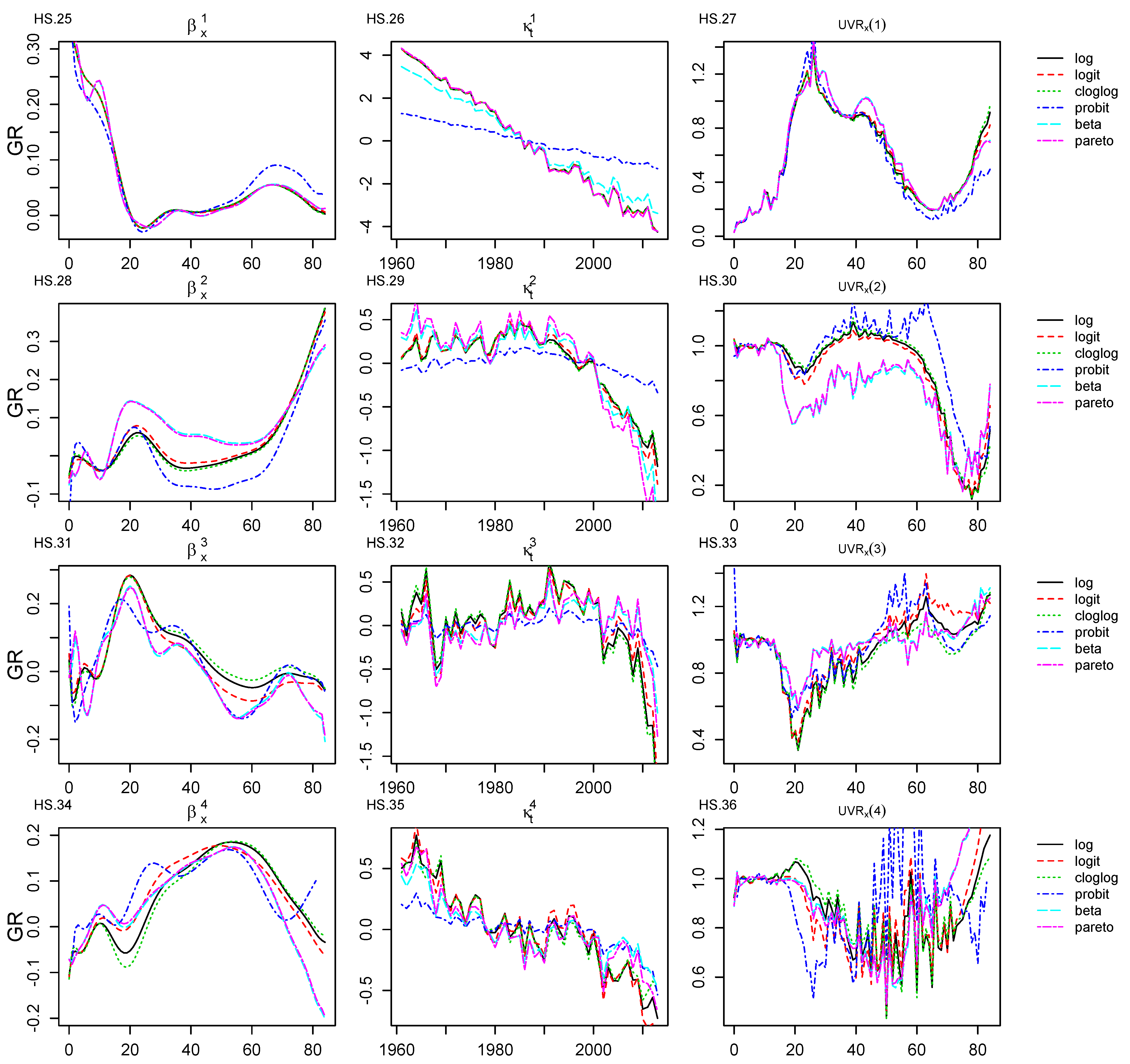
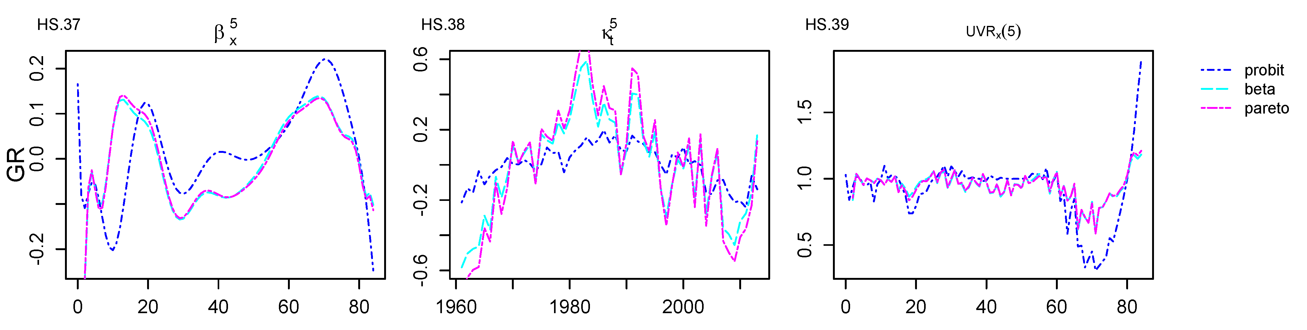
Table 1.
Link functions transformations of the HS model.
| Dist | Link Name | Link Function | Mean Function |
|---|---|---|---|
| Binomial | Logit | ||
| Cloglog | |||
| Probit | |||
| Inverse CDF | , if | ||
| , if | |||
| , if |
Table 2.
Optimum parameters for each HS model extension structure for the E&W dataset.
| Country: E&W | Years: 1841–2016 | Ages: 0–89 (Years) | |||||||
|---|---|---|---|---|---|---|---|---|---|
| Model | |||||||||
| HS_log | 54.50 | 29 | 5 | 4 | 2 | - | - | - | - |
| HS_lgt | 55.19 | 30 | 5 | 14 | 2 | - | - | - | - |
| HS_cll | 6.40 | 30 | 5 | 14 | 2 | - | - | - | - |
| HS_prbt | 9.26 | 30 | 5 | 10 | 2 | - | - | - | - |
| HS_beta | 4.13 | 30 | 5 | 8 | 2 | 6.00 | 1.25 | 4.00 | 1.25 |
| HS_prt | 71.45 | 23 | 6 | 4 | 1 | 16.50 | 1.00 | 11.50 | 1.00 |
Table 3.
Optimum parameters for each HS model extension structure for the GR dataset.
| Country: Greece | Years: 1961–2013 | Ages: 0–84 (Years) | |||||||
|---|---|---|---|---|---|---|---|---|---|
| Model | |||||||||
| HS_log | 2.55 | 16 | 4 | 8 | 1 | - | - | - | - |
| HS_lgt | 2.52 | 16 | 4 | 8 | 1 | - | - | - | - |
| HS_cll | 2.58 | 16 | 4 | 8 | 1 | - | - | - | - |
| HS_prbt | 0.21 | 16 | 5 | 8 | 1 | - | - | - | - |
| HS_beta | 2.18 | 20 | 5 | 8 | 1 | 1.25 | 0.50 | 1.00 | 0.25 |
| HS_prt | 3.37 | 20 | 5 | 8 | 1 | 4.00 | 1.00 | 7.00 | 1.00 |
Table 4.
Results of the quantitative tests for E&W mortality dataset.
| Model | npar | Log-Likelihood | AIC | BIC | MSPE (%) | MAPE (%) | |
|---|---|---|---|---|---|---|---|
| HS_log | 29 | 1598 | −135,970.84 | 275,137.68 | 287,394.81 | 0.329 | 3.696 |
| HS_lgt | 30 | 1634 | −125,713.76 | 254,695.52 | 267,228.78 | 0.336 | 3.694 |
| HS_cll | 30 | 1634 | −168,056.21 | 339,566.43 | 352,813.03 | 0.449 | 4.707 |
| HS_prbt | 30 | 1622 | −115,111.76 | 233,467.52 | 245,908.73 | 0.346 | 3.693 |
| HS_beta | 30 | 1343 | −129,916.62 | 262,519.24 | 272,820.45 | 0.381 | 3.945 |
| HS_prt | 23 | 1492 | −113,143.64 | 229,271.28 | 240,715.35 | 0.346 | 3.596 |
Table 5.
Results of the quantitative tests for well-known stochastic mortality models against HS_prt for E&W dataset.
Table 5.
Results of the quantitative tests for well-known stochastic mortality models against HS_prt for E&W dataset.
| Model | npar | Log-Likelihood | AIC | BIC | MSPE (%) | MAPE (%) |
|---|---|---|---|---|---|---|
| LC | 354 | −1,075,745.35 | 2,152,198.70 | 2,154,913.98 | 7.131 | 18.473 |
| RH | 707 | −553,002.06 | 1,107,418.13 | 1,112,841.02 | 5.369 | 14.896 |
| APC | 528 | −1,157,738.25 | 2,316,532.50 | 2,320,582.42 | 20.541 | 23.522 |
| PL | 880 | −762,205.25 | 1,526,170.51 | 1,532,920.37 | 9.136 | 15.737 |
| HS_log | 1598 | −135,970.84 | 275,137.68 | 287,394.81 | 0.329 | 3.696 |
| HS_prt | 1492 | −113,143.64 | 229,271.28 | 240,715.35 | 0.346 | 3.596 |
Table 6.
Results of the quantitative tests for the Greek mortality dataset.
| Model | npar | Log-Likelihood | AIC | BIC | MSPE (%) | MAPE (%) | |
|---|---|---|---|---|---|---|---|
| HS_log | 16 | 447 | −20,176.13 | 41,246.26 | 44,112.84 | 4.109 | 10.115 |
| HS_lgt | 16 | 447 | −20,069.65 | 41,033.29 | 43,899.88 | 4.080 | 10.065 |
| HS_cll | 16 | 447 | −20,133.42 | 41,160.85 | 44,027.43 | 4.104 | 10.079 |
| HS_prbt | 16 | 516 | −19,569.21 | 40,170.43 | 43,479.50 | 4.078 | 10.074 |
| HS_beta | 20 | 540 | −19,358.74 | 39,797.48 | 43,260.47 | 3.444 | 9.515 |
| HS_prt | 20 | 540 | −19,353.29 | 39,786.59 | 43,249.58 | 3.449 | 9.498 |
Table 7.
Results of the quantitative tests for well-known stochastic mortality models against HS_prt for GR dataset.
Table 7.
Results of the quantitative tests for well-known stochastic mortality models against HS_prt for GR dataset.
| Model | npar | Log-Likelihood | AIC | BIC | MSPE (%) | MAPE (%) |
|---|---|---|---|---|---|---|
| LC | 221 | −21,213.44 | 42,868.89 | 44,286.15 | 4.287 | 11.379 |
| RH | 441 | −18,633.10 | 38,148.19 | 40,976.30 | 3.790 | 9.460 |
| APC | 272 | −21,317.67 | 43,179.33 | 44,923.65 | 5.405 | 12.715 |
| PL | 378 | −19,113.68 | 38,983.36 | 41,407.45 | 5.395 | 10.371 |
| HS_log | 447 | −20,176.13 | 41,246.26 | 44,112.84 | 4.109 | 10.115 |
| HS_prt | 540 | −19,353.29 | 39,786.59 | 43,249.58 | 3.449 | 9.498 |
Table 8.
Optimum parameters for HS_prt structure for the E&W and GR shorter datasets.
| Model: HS_prt | |||||||||||
|---|---|---|---|---|---|---|---|---|---|---|---|
| Country | Years | Ages | |||||||||
| E&W | 1841–2006 | 0–89 | 56.58 | 29 | 6 | 4 | 1 | 15 | 1.00 | 11.50 | 1.00 |
| GR | 1961–2003 | 0–84 | 1.55 | 20 | 3 | 8 | 1 | 5.50 | 1.00 | 11.50 | 1.00 |
Table 9.
Results of the percentage error tests for predicted mortality rates of 10 years out-of-sample for well-known stochastic mortality models against HS_prt for E&W dataset.
Table 9.
Results of the percentage error tests for predicted mortality rates of 10 years out-of-sample for well-known stochastic mortality models against HS_prt for E&W dataset.
| MSPE (%) | MAPE (%) | |||
|---|---|---|---|---|
| RWD | ARIMA | RWD | ARIMA | |
| HS_prt | 3.206 | 5.550 | 13.219 | 18.852 |
| HS_log | 3.221 | 7.135 | 13.271 | 20.800 |
| RH | 271.861 | 271.861 | 58.085 | 58.085 |
| LC | 29.508 | 29.509 | 49.838 | 49.837 |
| PL | 586.784 | 371.845 | 62.748 | 55.635 |
| APC | 86.494 | 84.316 | 46.192 | 46.131 |
Table 10.
Results of the percentage error tests for predicted mortality rates of 10 years out-of-sample for well-known stochastic mortality models against HS_prt for GR dataset.
Table 10.
Results of the percentage error tests for predicted mortality rates of 10 years out-of-sample for well-known stochastic mortality models against HS_prt for GR dataset.
| MSPE (%) | MAPE (%) | |||
|---|---|---|---|---|
| RWD | ARIMA | RWD | ARIMA | |
| HS_prt | 8.446 | 8.549 | 14.961 | 15.067 |
| HS_log | 8.691 | 10.390 | 15.332 | 15.857 |
| RH | 8.361 | 8.581 | 15.440 | 15.275 |
| LC | 10.398 | 10.333 | 20.320 | 20.964 |
| PL | 8.860 | 11.163 | 18.402 | 15.148 |
| APC | 10.054 | 10.077 | 21.364 | 21.599 |
Publisher’s Note: MDPI stays neutral with regard to jurisdictional claims in published maps and institutional affiliations. |
© 2022 by the authors. Licensee MDPI, Basel, Switzerland. This article is an open access article distributed under the terms and conditions of the Creative Commons Attribution (CC BY) license (https://creativecommons.org/licenses/by/4.0/).
Share and Cite
MDPI and ACS Style
Sagianou, A.; Hatzopoulos, P. Extensions on the Hatzopoulos–Sagianou Multiple-Components Stochastic Mortality Model. Risks 2022, 10, 131. https://doi.org/10.3390/risks10070131
AMA Style
Sagianou A, Hatzopoulos P. Extensions on the Hatzopoulos–Sagianou Multiple-Components Stochastic Mortality Model. Risks. 2022; 10(7):131. https://doi.org/10.3390/risks10070131
Chicago/Turabian StyleSagianou, Aliki, and Peter Hatzopoulos. 2022. "Extensions on the Hatzopoulos–Sagianou Multiple-Components Stochastic Mortality Model" Risks 10, no. 7: 131. https://doi.org/10.3390/risks10070131
Note that from the first issue of 2016, this journal uses article numbers instead of page numbers. See further details here.