
Modelling and Simulation/Optimization of Austria’s National Multi-Energy System with a High Degree of Spatial and Temporal Resolution

 and
and
Abstract
:1. Introduction
- A spatial and timely compensation of energy;
- An increase in flexibility for both demand and generation in an energy system;
- The ability to cope with high instantaneous penetration of RES;
- Curtailment of RES as ultima-ratio.
1.1. Literature Overview and Research Need
1.1.1. MES Simulation and Optimization Approaches
- More than two individual network levels;
- No energy transfers across various network levels, since only step-by-step energy transfer via each network level is possible (energy must always flow via each network level without skipping network levels);
- A lack of selectable control strategies for both sector coupling and energy storage options;
- Implementation of further components of an energy system is only possible with high programming effort.
1.1.2. MES Investigations on National Level
1.1.3. Research Need
- Based on the scientific gap, how should an MES simulation framework be designed to cope with a national MES and various other research questions with a high degree of both spatial and temporal resolution?
- What steps have to be taken to model Austria’s national energy system with detailed spatial and temporal resolution?
- What are the effects on power infrastructure based on #mission2030 renewable energy sources expansion, considering different modes of flexibility operation and power load flow optimization?
1.2. Problem Description
- The flexible depiction of various network levels of all energy carriers (power, gas, heat), independent of spatial resolution. This should enable a large range of spatial resolution to be able to depict various areas, from single consumers up to the state level.
- The possibility to assign various flexibility options, such as sector coupling technologies, storage options, demand-side management (DSM), and operation-flexible power plants. This should include the possibility of flexibly adding any further components to expand the MES framework’s functionality. Flexibilities may operate, e.g., as load following units or with various optimization-based operation strategies, such as maximizing profits or maximizing the degree of self-sufficiency in a specified area.
- State of art load flow consideration via adequate load flow calculation for all considered energy carriers. Depending on the user’s selection, power flow simulation or optimal power flow load flow calculations should be selectable for the power grid.
- Suitable approaches and data to be found to achieve a detailed spatial resolution. This includes consumption and generation data for all energy carriers. If data are not available in low spatial resolution, a suitable approach must be found to distribute general data towards smaller entities.
- Currently, no models of Austria’s power, natural gas, and district heating energy infrastructure are openly available. To allow for the consideration of real grid properties, an energy grid model must be developed, based on available data to depict the Austrian energy infrastructure.
2. Methodology
2.1. HyFlow
2.1.1. General Modelling Structure
2.1.2. Input Data
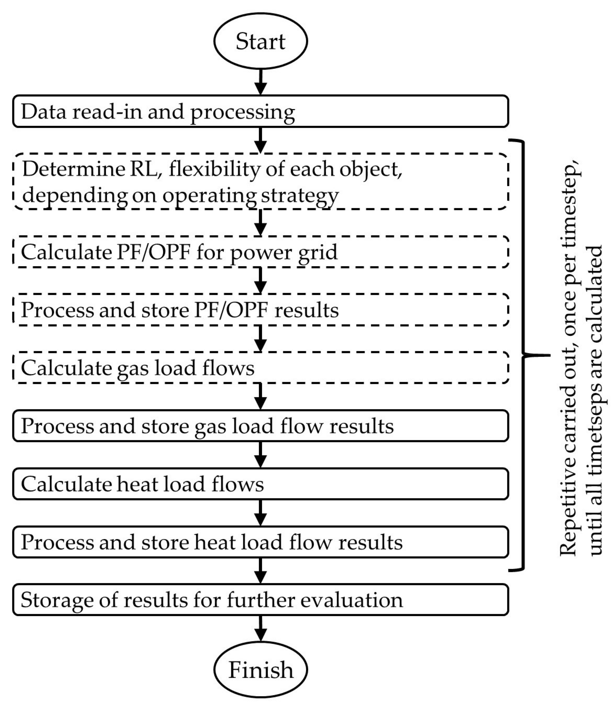
2.1.3. Calculation Procedure and Grid Simulation
Determination of RL
Power Grid PF or OPF
Gas and Heat Load Flow Calculation
Process and Storage of Results
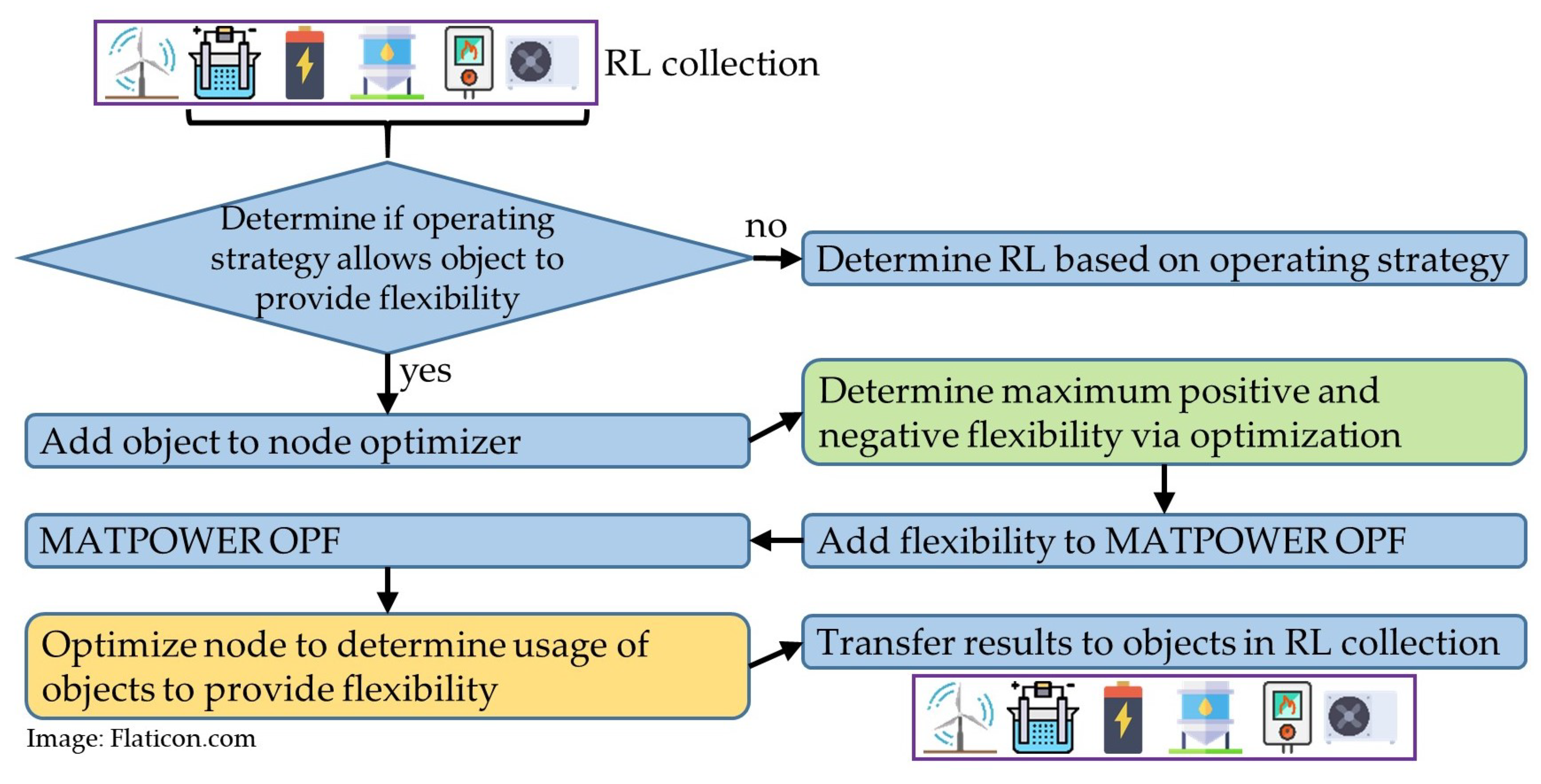
2.1.4. Implementation and Usage of Flexibility Options
2.2. Austrian MES Modelling
2.2.1. Power Grid
2.2.2. Natural Gas Grid
2.2.3. Heat Grid
2.2.4. Model of Austrian Natural Gas and Power Grid
2.2.5. Spatial Data Distribution
2.2.6. Temporally Resolved Consumption Data
2.2.7. Temporally Resolved Generation Data
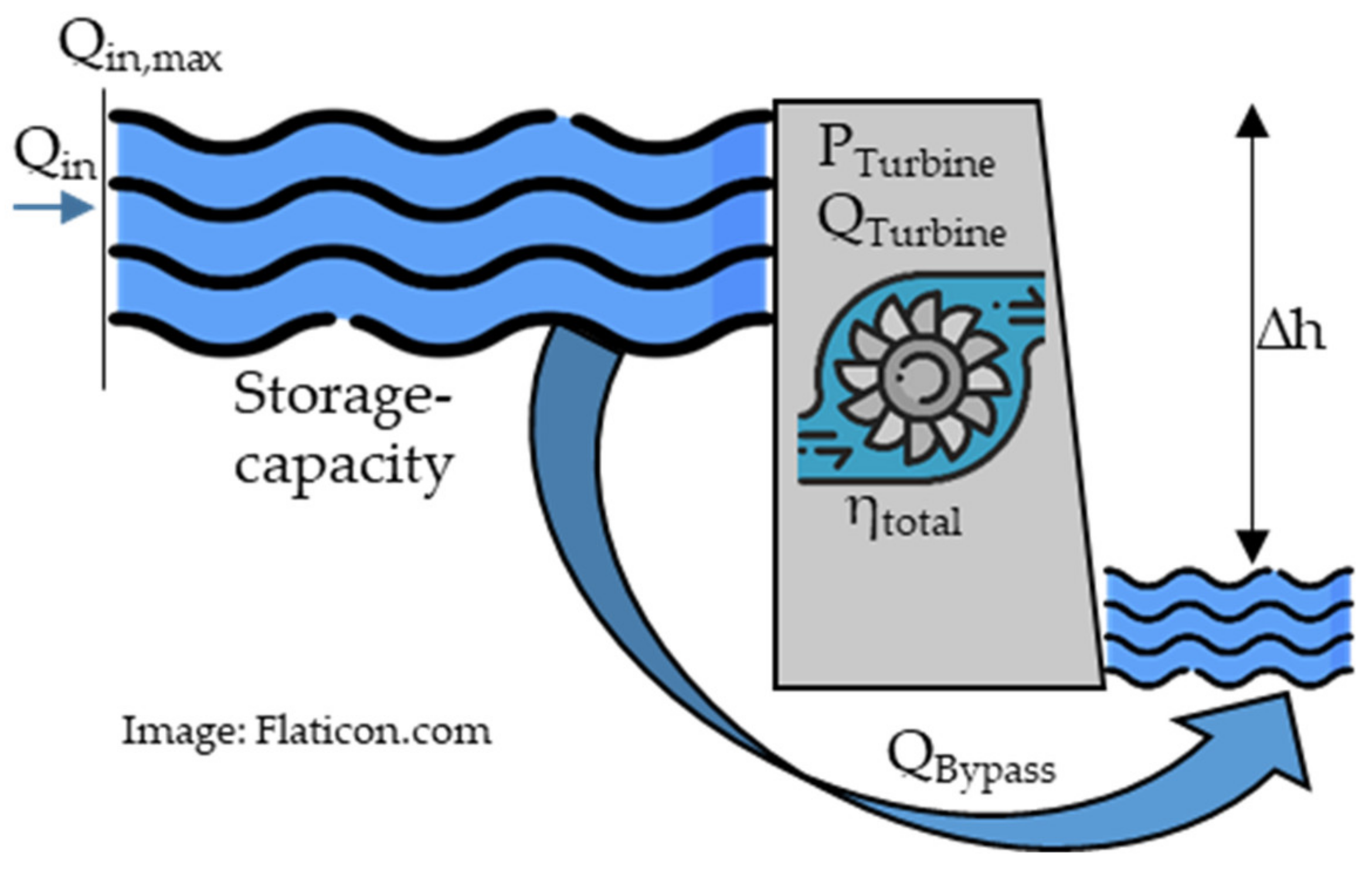
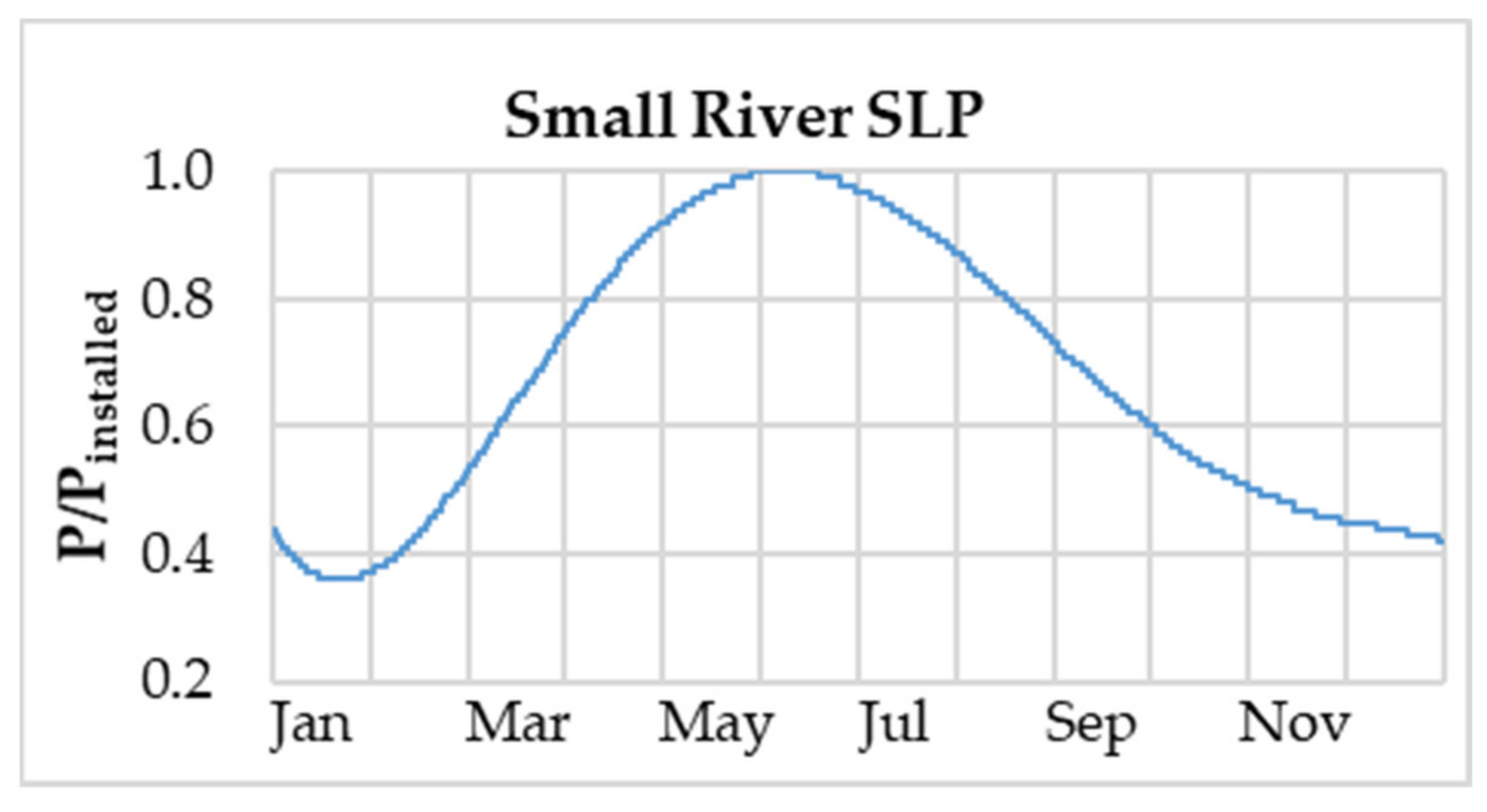
Hydro Run-Off and Storage Power Station
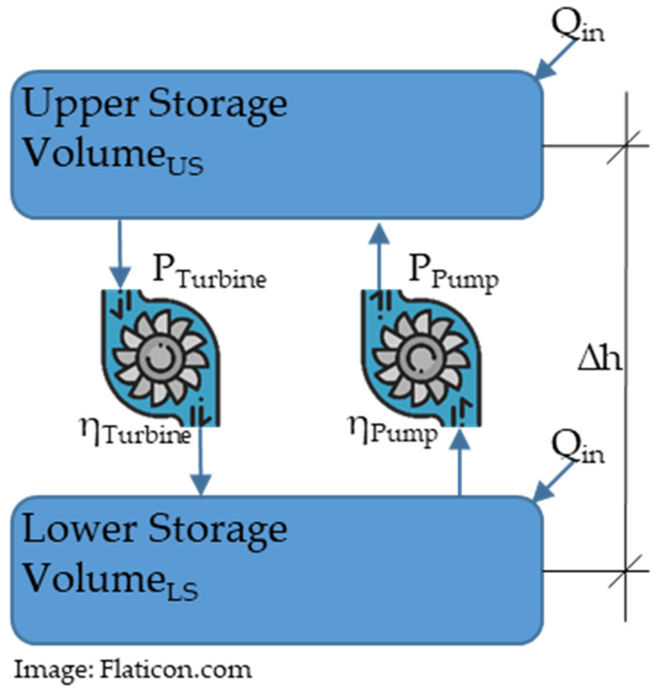
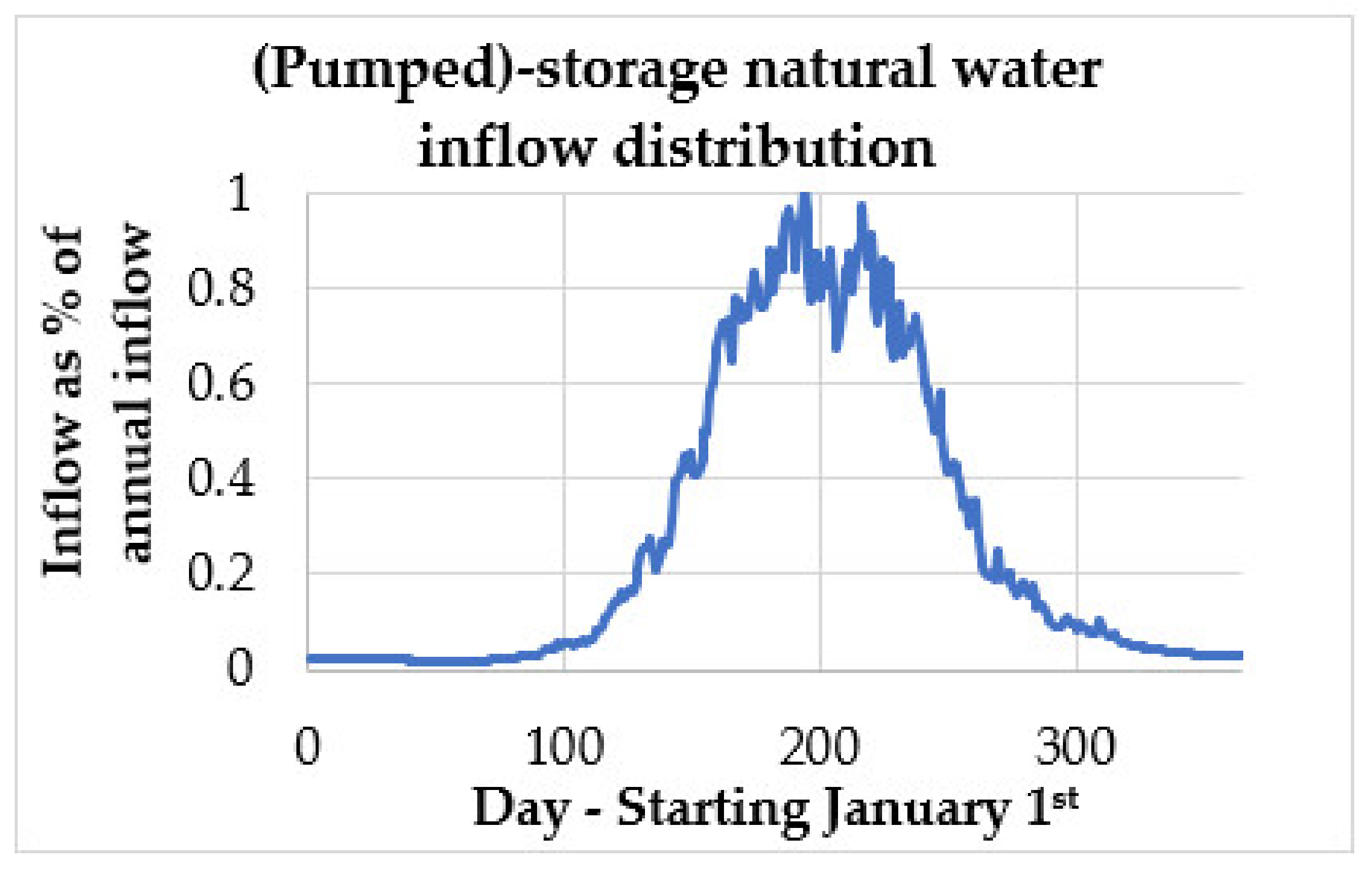
(Pumped)-Storage Hydropower Plant
Biomass Combined Heat and Power (CHP) and Biogas Power Plants
Photovoltaics
Wind
Thermal Generation
2.2.8. Power Exchange with Neighboring Countries
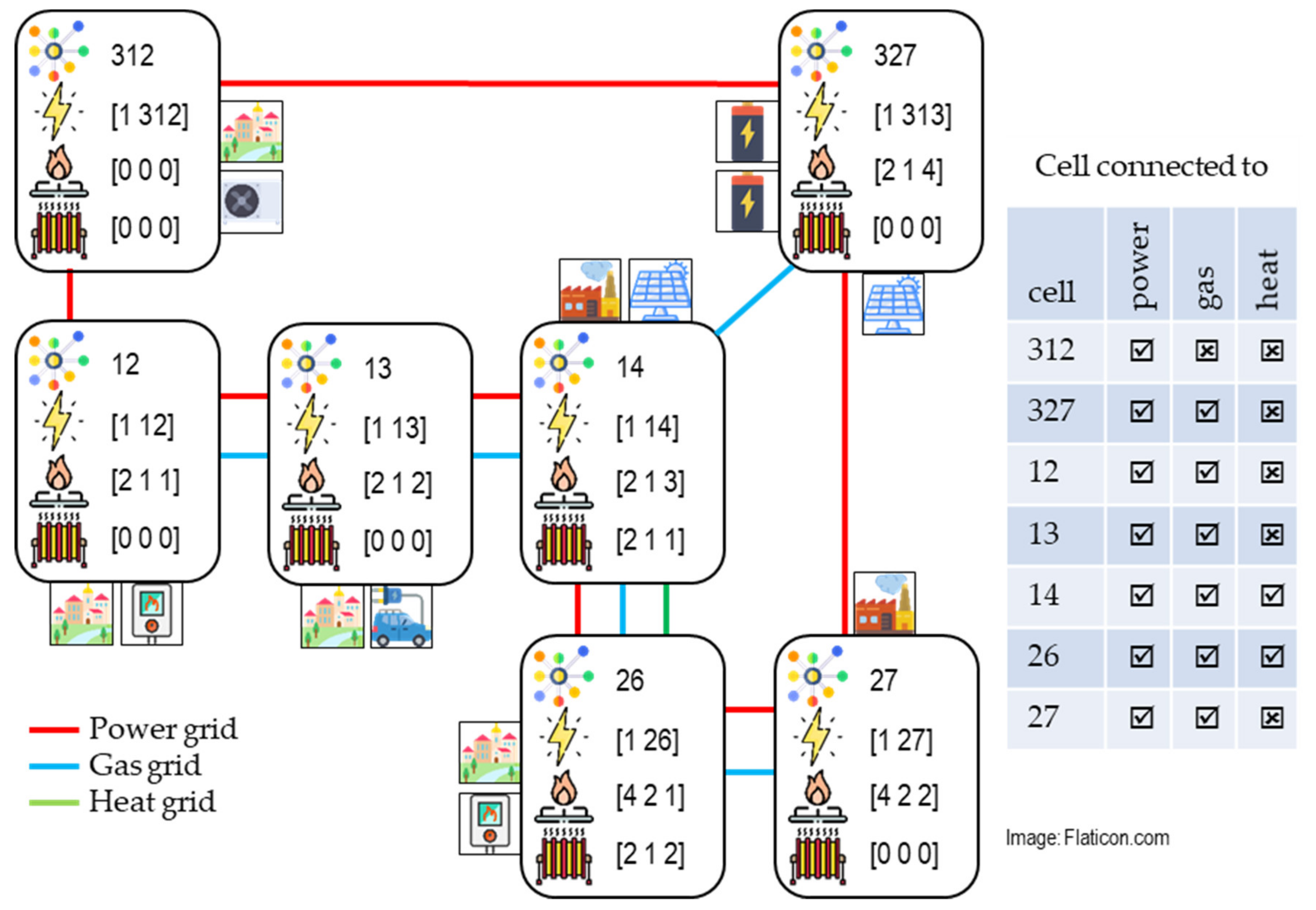
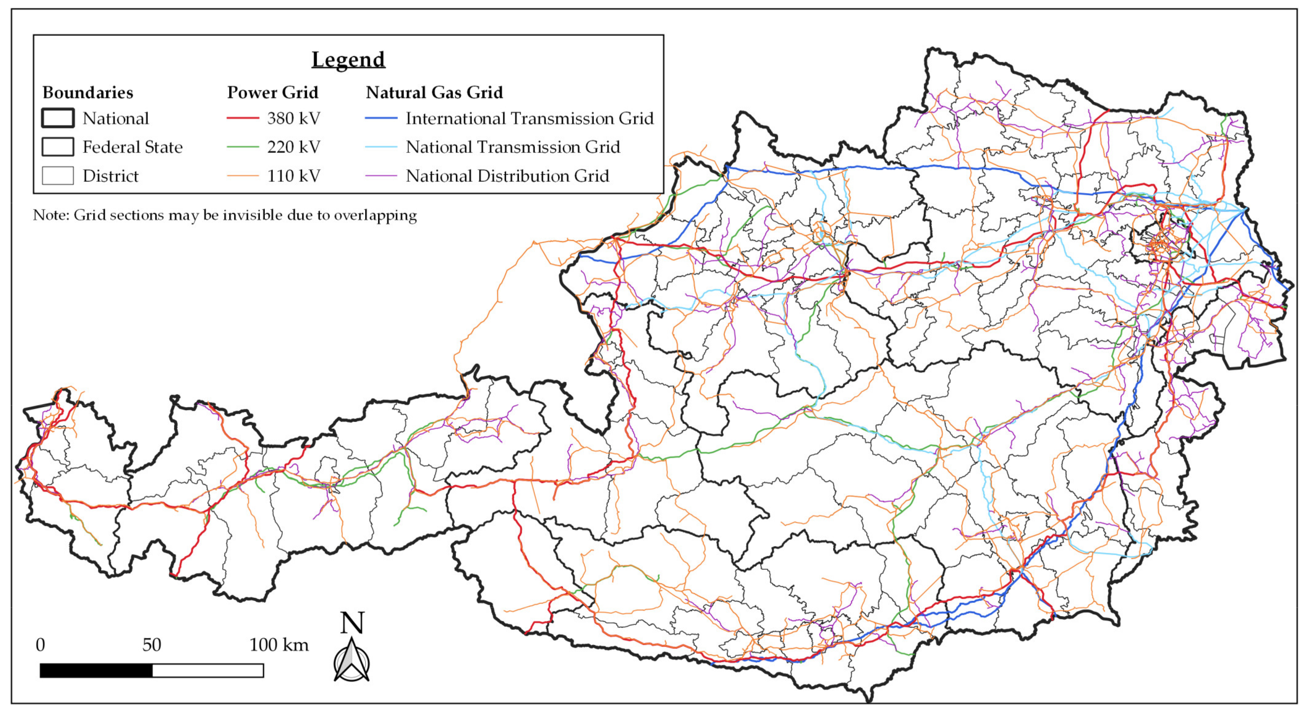
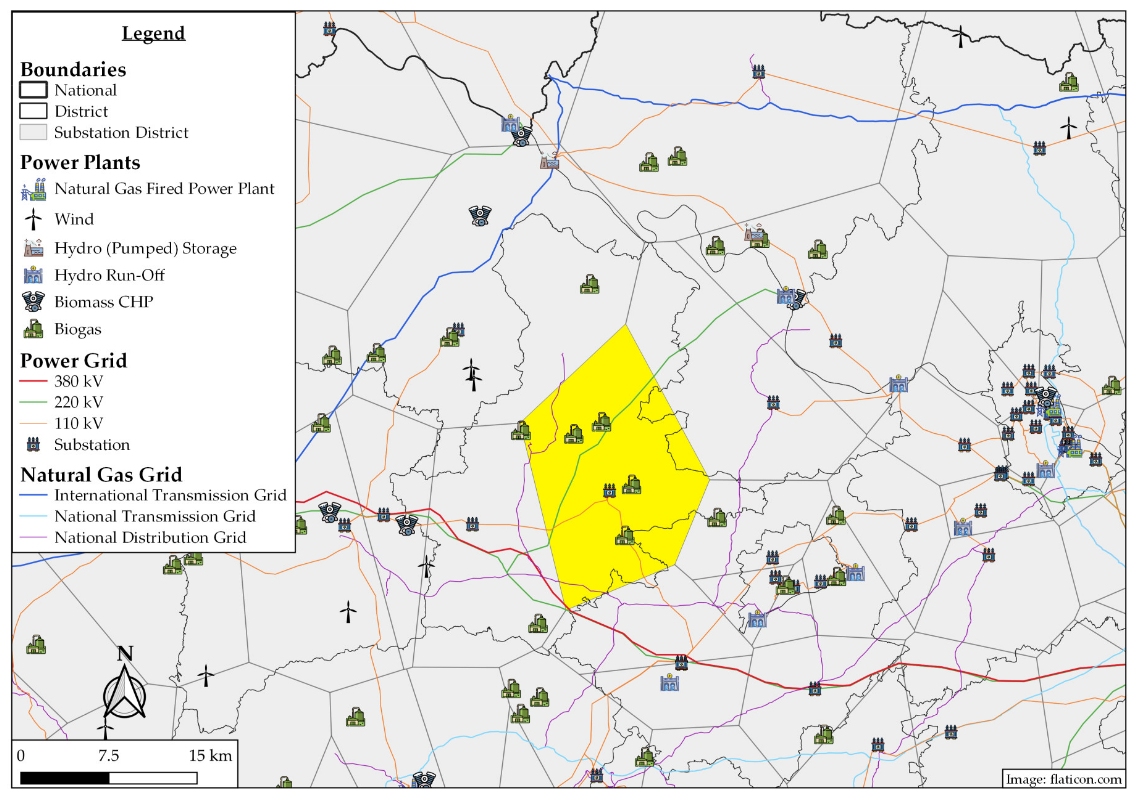
2.2.9. Example of Energy Infrastructure Depiction
3. Scenarios
- Since power, gas, and heat consumption are based on past data, sufficient studies need to be found to estimate the energy consumption in 2030. Austria’s Umweltbundesamt (UBA) [99] estimates energy consumption in the years 2020, 2030, and 2050, based on the year 2015. Power demand is expected to remain stable between 2015 and 2020 and then increase between seven and thirty per cent, depending on the scenario. Electric vehicles, heat pumps, and electrolysis are seen as major drivers of power consumption growth. Since these consumers are additionally considered in each following scenario, we assume that the power demand will stay constant without. Depending on the scenario, a slight increase or decrease in natural gas consumption is assumed by UBA; therefore, we assume constant consumption [99]. Based on #mission2030 targets, thermal renovation of existing buildings should be doubled to two per cent per year, from current levels of around one per cent [5]. If a 50% heat demand reduction through a thermal renovation is assumed, heat demand might drop by thirteen per cent, until 2030. The assumption of 50% heat demand reduction seems reasonable since subsidiaries are granted if more than 40% heat demand reduction is achieved [100]. The 13% heat reduction is between both UBA scenarios (WAM, WEM) for the final energy consumption of buildings [99].
- The number of electric vehicles in each SSD is determined based on vehicle registration data and trends in each federal state [101]. The share of electric vehicles in 2030 is expected to be 20%, based on scenarios in [102]. In Austria, a car is used for an average of 13,700 km per year. Based on the average consumption of 20 kWh/100 km, an annual electric energy demand per car of about 2750 kWh can be expected [103,104]. The temporal charging characteristic is scenario-dependent and can be explained in the following subchapters. All electric vehicles account for approximately 3 TWh of additional power consumption.
- The share of heat pumps for each SSD is determined based on the share of ambient heat usage for heating purpose divided by an assumed coefficient of performance of three [55]. Heat pump usage might increase by six-fold until 2030 based on [105]. The mode of operation depends on the scenario. All heat pumps account for approximately 1.9 TWh of additional power consumption.
- For every fourth household, battery energy storage with a storage capacity of 8 kWh, charging–discharging power of 2 kW, and an input–output efficiency of 90% [106] is implemented with a scenario-dependent mode of operation.
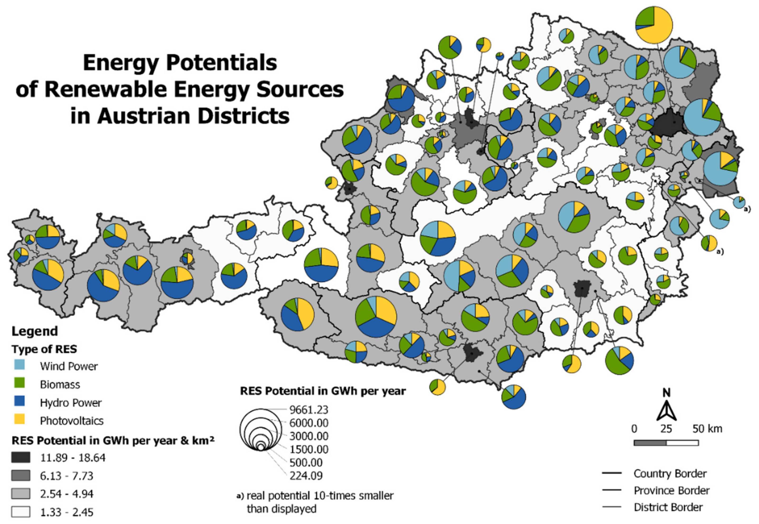
- Renewable energy sources are expanded according to plans of the federal government, shown in Table 3.
3.1. Scenario 1—BAU
3.2. Scenario 2—Demand Optimization
3.3. Scenario 3—Demand Optimization and Flexibility
- Subsidized forms of power generation, such as biogas, biomass CHP, wind, photovoltaics, and small-scale hydropower with 10 EUR/MWh;
- Large-scale hydropower 50 EUR/MWh;
- Flexibilities (gas turbine and CHP and (pumped)-storage hydropower) and import/export with 100 EUR/MWh.
4. Results
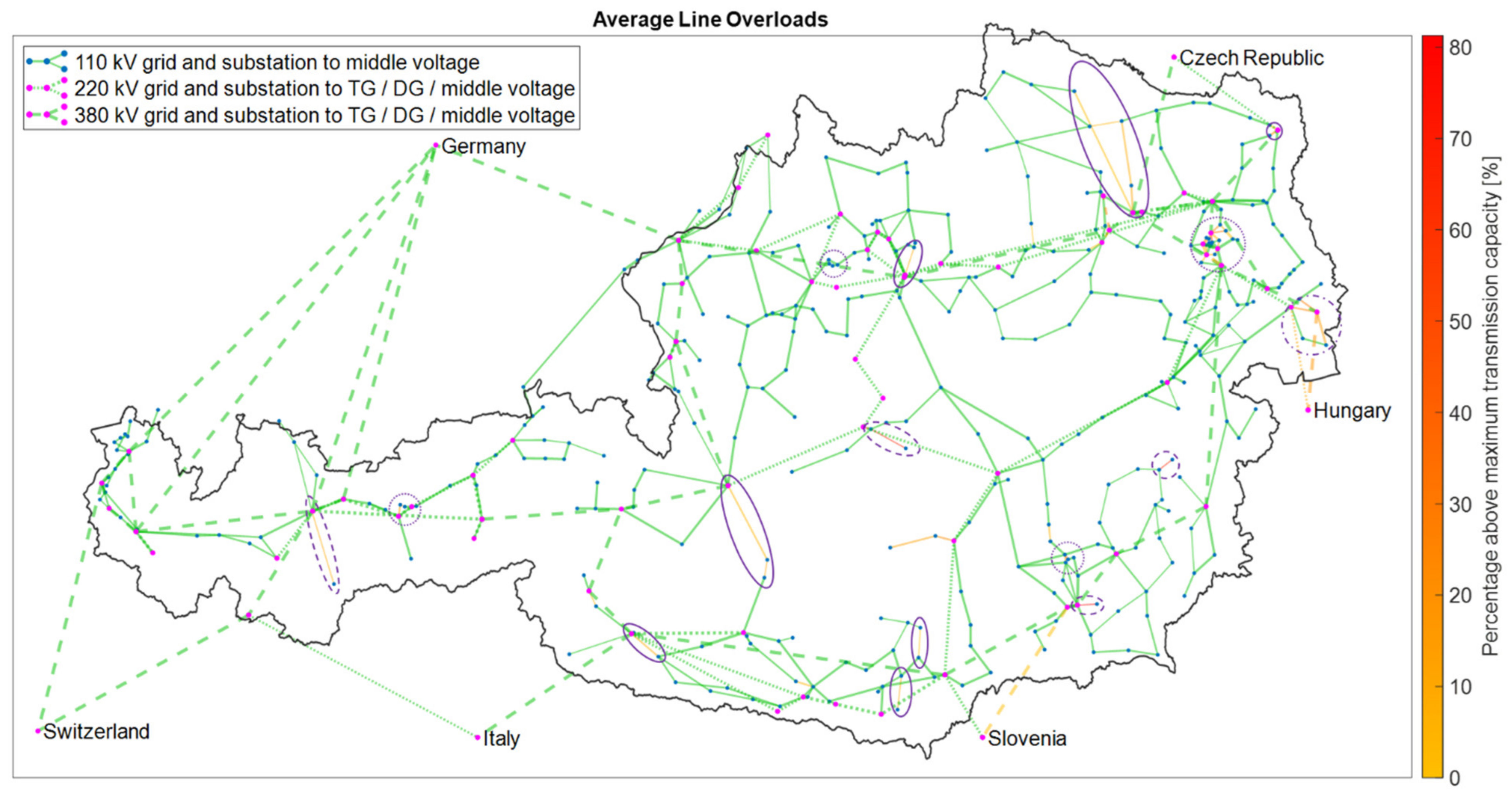
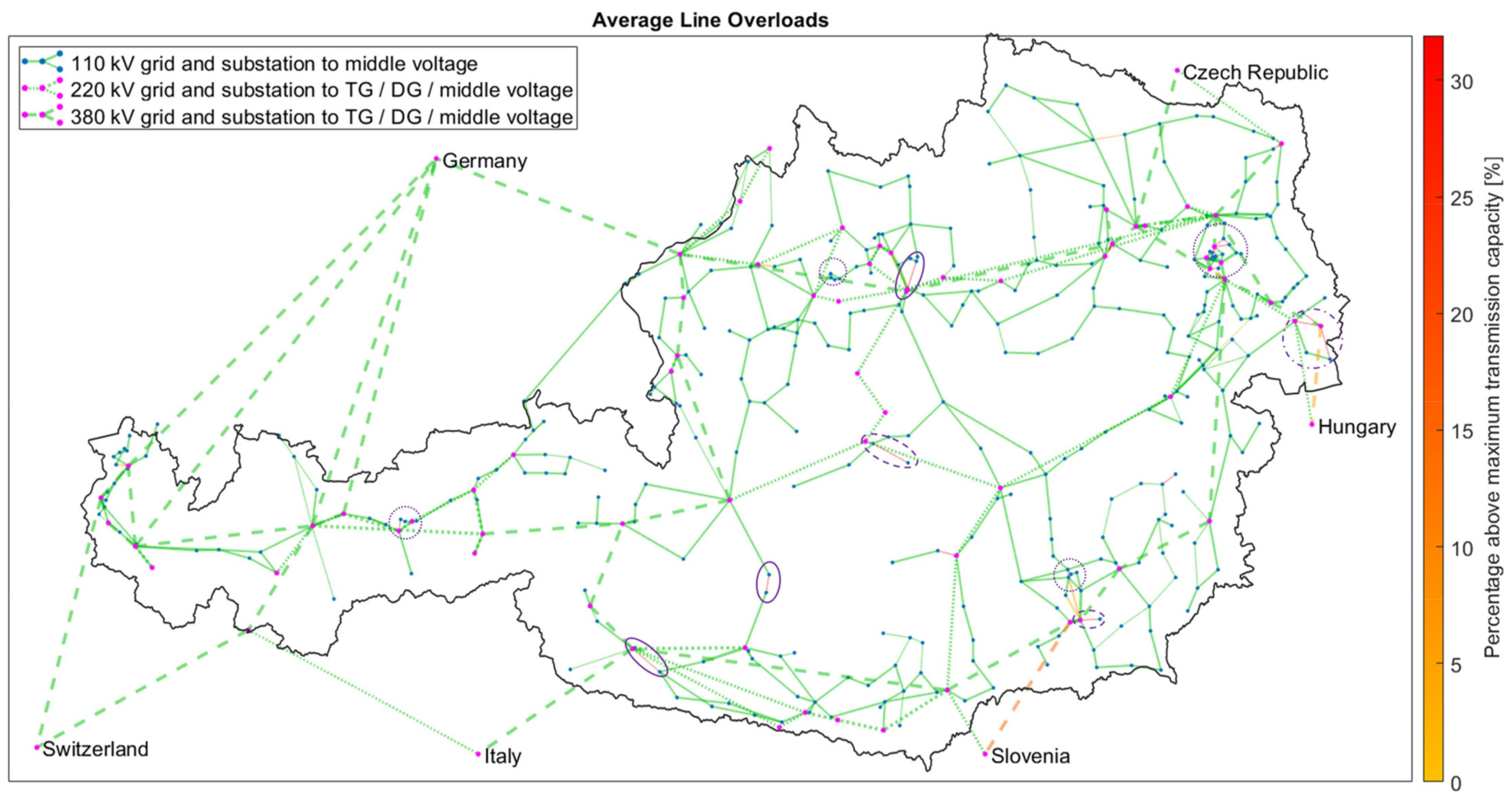
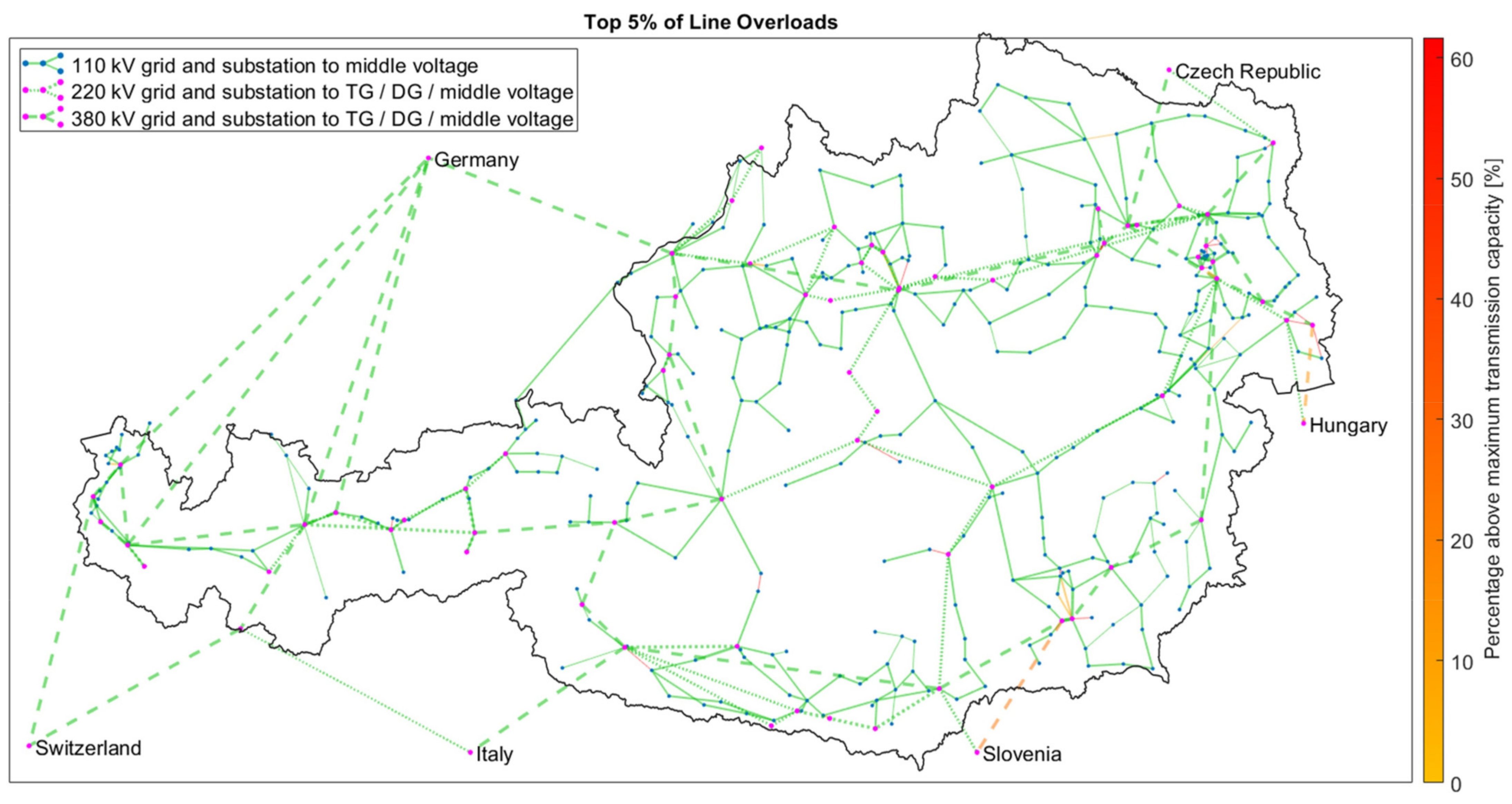
- Continuous purple line—sections with low transmission capacity, e.g., single three-wire system;
- Dotted purple line—overloaded lines in urban areas;
- Dashed purple line—branch line with low transmission capacity in combination with either high potential of RES generation or demand;
- Dashed-dotted purple line—high potential of RES expansion.

5. Discussion
5.1. MES Model of Austria
5.2. Simulation Results
6. Conclusions and Future Outlook
Author Contributions
Funding
Conflicts of Interest
Abbreviations
| APG | Austrian Power Grid |
| CHP | combined heat and power |
| DG | distribution grid |
| EC | energy carrier |
| GtH | gas to heat |
| GtPH | gas to power and heat |
| HtP | heat to power |
| MES | multi-energy system |
| MESS | multi-energy system simulator |
| OPF | optimal power flow |
| PF | power flow |
| PtGH | power to gas and heat |
| PtH | power to heat |
| RES | renewable energy source |
| RL | residual load |
| SC | sector coupling |
| SLP | standardized Load Profile |
| SSD | sub-station district |
| TG | transmission grid |
| UBA | Umweltbundesamt (Federal Environment Agency) |
Appendix A. Node Optimization

Appendix A.1. Input Data

| Parameter | Type | Description |
|---|---|---|
| P_RL_Set | scalar | Residual load setting for the current time step. |
| t | scalar | Duration of one time step [h]. |
| Converter | matrix | Defines properties of each converter. Each row represents one converter. [FP, FH, FG, TP, TH, TG, MinP, MaxP, Ramp, PPrevPeriod] FP—convert from power (1 or 0). FH—convert from heat (1 or 0). FG—convert from gas (1 or 0). TP—convert to power (η in [1]). TH—convert to heat (η in [1]). TG—convert to gas (η in [1]). MinP—minimum power [W]. MaxP—maximum power [W]. Ramp—ramp rate based on MaxP. PPrevPeriod—power of previous period [W]. |
| P_Storage H_Storage G_Storage | matrix | Defines properties of each storage. Each row represents one storage. For power, heat, and gas, individual matrices have to be set up with the following structure. [LP, MinSL, MaxSL, ISL, ηIn, MinIn, MaxIn, ηOut, MinOut, MaxOut] LP—storage loss per period [1/h]. MinSL—minimum allowed storage level [Wh]. MaxSL—maximum allowed storage level [Wh]. ISL—initial storage level [Wh]. ηIn—input efficiency [1]. MinIn—minimum input power [W]. MaxIn—maximum input power [W]. ηOut—output efficiency [1]. MinOut—minimum output power [W]. MaxOut—maximum output power [W]. |
| P_DSM H_DSM G_DSM | matrix | Defines properties of each DSM. Each row represents one DSM. For power, heat, and gas, individual matrices have to be set up with the following structure. [MinP, MaxP] MinP—minimum feed-in (demand) or maximum feed-out (generation) power. MaxP—maximum feed-in (demand) or minimum feed-out (generation) power. |
| eVehicle | vector | Defines parameters for electric vehicles. [EC, CP, NoP, SB_1, EB_1, SB_2, EB_2] EC—energy to be charged within NoP [Wh]. CP—charging power [W]. NoP—number of time steps before charging of EC must be finished (e.g., one day). SB_1, SB_2—the start of the charging break period. EB_1, EB_2—the end of the charging break period. |
| P_Price H_Price G_Price | vector | The number of rows is equivalent to the forecasting period. A separate vector must be defined for each energy carrier’s price. |
| P_RL H_RL G_RL | vector | The number of rows is equivalent to the forecasting period. A separate vector must be defined for each energy carrier’s residual load [W]. |
| G_Connect H_Connect | scalar | Indicates if the node is connected (variable = 1) to gas/heat grid or not (variable = 0). |
| ops | vector | Contains settings for the Gurobi optimizer. |
Appendix A.2. Node Optimization Target Function (TF)
Appendix A.3. Flexibility Determination Target Function
Appendix A.4. Results
Appendix B. Measurement Points for Small Hydropower Plant SLP
| Federal State | Measurement Point # | Name |
|---|---|---|
| Vorarlberg | 200105 | Garsella |
| Tyrol | 230706 | In der Au |
| Salzburg | 203265 | Schweighofbrücke |
| Carinthia | 213389 | Kaunz |
| Styria | 211029 | Anger |
| Upper Austria | 204784 | Riedau |
| Lower Austria | 208041 | Hollenstein |
| Burgenland | 210039 | Piringsdorf (Pfarrbrücke) |
| Vienna | None | None |
Appendix C. Measurement Points for Natural Inflow Curve for (Pumped)-Storage Hydropower Plants
| Measurement Point Name | Measurement Point # | Elevation [m] |
|---|---|---|
| Gepatschalm | 230300 | 1895 |
| Vent (oberhalb Niedertalbach) | 201350 | 1891 |
| Obergurgl | 201376 | 1879 |
| Neukaser | 201996 | 1786 |
| Innergschlöß | 212068 | 1686 |
| Kees | 203893 | 2040 |
References
- European Commission. The European Green Deal, Brussels, 2019. Available online: https://eur-lex.europa.eu/resource.html?uri=cellar:b828d165-1c22-11ea-8c1f-01aa75ed71a1.0002.02/DOC_1&format=PDF (accessed on 12 January 2022).
- European Commission. What is the European Green Deal? Brussels, 2019. Available online: https://ec.europa.eu/commission/presscorner/detail/en/fs_19_6714 (accessed on 12 November 2021).
- European Commission. Fit for 55: Delivering the EU’s 2030 Climate Target on the Way to Climate Neutrality, Brussels, 2021. Available online: https://eur-lex.europa.eu/legal-content/EN/TXT/PDF/?uri=CELEX:52021DC0550&from=DE (accessed on 12 November 2021).
- Bundeskanzleramt. Aus Verantwortung für Österreich: Regierungsprogramm 2020–2024, Wien, 2020. Available online: https://www.bundeskanzleramt.gv.at/dam/jcr:7b9e6755-2115-440c-b2ec-cbf64a931aa8/RegProgramm-lang.pdf (accessed on 11 November 2021).
- Bundesministerium Nachhaltigkeit und Tourismus; Bundesministerium Verkehr Innovation und Technologie. #Mission2030: Die Österreichische Klima- und Energiestrategie, Wien, 2018. Available online: https://www.bundeskanzleramt.gv.at/dam/jcr:903d5cf5-c3ac-47b6-871c-c83eae34b273/20_18_beilagen_nb.pdf (accessed on 12 January 2022).
- Mancarella, P. MES (multi-energy systems): An overview of concepts and evaluation models. Energy 2014, 65, 1–17. [Google Scholar] [CrossRef]
- Hansen, K.; Breyer, C.; Lund, H. Status and perspectives on 100% renewable energy systems. Energy 2019, 175, 471–480. [Google Scholar] [CrossRef]
- Sejkora, C.; Kühberger, L.; Radner, F.; Trattner, A.; Kienberger, T. Exergy as Criteria for Efficient Energy Systems—A Spatially Resolved Comparison of the Current Exergy Consumption, the Current Useful Exergy Demand and Renewable Exergy Potential. Energies 2020, 13, 843. [Google Scholar] [CrossRef] [Green Version]
- Bundesamt für Eich- und Vermessungswesen. Katalog Verwaltungsgrenzen (VGD)—Stichtagsdaten 1:5000; Bundesamt für Eich- und Vermessungswesen: Wien, Austria; Available online: https://www.data.gv.at/katalog/dataset/bev_verwaltungsgrenzenstichtagsdaten150000 (accessed on 15 February 2022).
- Klemm, C.; Vennemann, P. Modeling and optimization of multi-energy systems in mixed-use districts: A review of existing methods and approaches. Renew. Sustain. Energy Rev. 2021, 135, 110206. [Google Scholar] [CrossRef]
- Pfenninger, S.; Hawkes, A.; Keirstead, J. Energy systems modeling for twenty-first century energy challenges. Renew. Sustain. Energy Rev. 2014, 33, 74–86. [Google Scholar] [CrossRef]
- Bottecchia, L.; Lubello, P.; Zambelli, P.; Carcasci, C.; Kranzl, L. The Potential of Simulating Energy Systems: The Multi Energy Systems Simulator Model. Energies 2021, 14, 5724. [Google Scholar] [CrossRef]
- Lohmeier, D.; Cronbach, D.; Drauz, S.R.; Braun, M.; Kneiske, T.M. Pandapipes: An Open-Source Piping Grid Calculation Package for Multi-Energy Grid Simulations. Sustainability 2020, 12, 9899. [Google Scholar] [CrossRef]
- Weinand, J.M.; Scheller, F.; McKenna, R. Reviewing energy system modelling of decentralized energy autonomy. Energy 2020, 203, 117817. [Google Scholar] [CrossRef]
- Thurner, L.; Scheidler, A.; Schafer, F.; Menke, J.-H.; Dollichon, J.; Meier, F.; Meinecke, S.; Braun, M. Pandapower—An Open-Source Python Tool for Convenient Modeling, Analysis, and Optimization of Electric Power Systems. IEEE Trans. Power Syst. 2018, 33, 6510–6521. [Google Scholar] [CrossRef] [Green Version]
- Böckl, B.; Greiml, M.; Leitner, L.; Pichler, P.; Kriechbaum, L.; Kienberger, T. HyFlow—A Hybrid Load Flow-Modelling Framework to Evaluate the Effects of Energy Storage and Sector Coupling on the Electrical Load Flows. Energies 2019, 12, 956. [Google Scholar] [CrossRef] [Green Version]
- Kienberger, T.; Traupmann, A.; Sejkora, C.; Kriechbaum, L.; Greiml, M.; Böckl, B. Modelling, designing and operation of grid-based multi-energy systems. Int. J. Sustain. Energy Plan. Manag. 2020, 29, 7–24. [Google Scholar] [CrossRef]
- Greiml, M.; Fritz, F.; Kienberger, T. Increasing installable photovoltaic power by implementing power-to-gas as electricity grid relief—A techno-economic assessment. Energy 2021, 235, 121307. [Google Scholar] [CrossRef]
- FFG. SBM_Ind: Smart Business Models for Industry. Available online: https://projekte.ffg.at/projekt/3093356 (accessed on 13 November 2021).
- Farshidian, B.; Ghahnavieh, A.R. A comprehensive framework for optimal planning of competing energy hubs based on the game theory. Sustain. Energy Grids Netw. 2021, 27, 100513. [Google Scholar] [CrossRef]
- Cheng, Y.; Zhang, P.; Liu, X. Collaborative Autonomous Optimization of Interconnected Multi-Energy Systems with Two-Stage Transactive Control Framework. Energies 2020, 13, 171. [Google Scholar] [CrossRef] [Green Version]
- Sejkora, C.; Kühberger, L.; Radner, F.; Trattner, A.; Kienberger, T. Exergy as criteria for efficient energy systems—Maximising energy efficiency from resource to energy service, an Austrian case study. Energy 2022, 239, 122173. [Google Scholar] [CrossRef]
- Wagner & Elbling GmbH. ONE100: Österreichs Nachhaltiges Energiesystem—100% Dekarbonisiert, Wien, 2021. Available online: https://www.aggm.at/files/get/b2327a5f19bc53c7fa0f2ae1dcd4edb1/ONE100_Kurzfassung.pdf (accessed on 14 November 2021).
- Aryanpur, V.; O’Gallachoir, B.; Dai, H.; Chen, W.; Glynn, J. A review of spatial resolution and regionalisation in national-scale energy systems optimisation models. Energy Strategy Rev. 2021, 37, 100702. [Google Scholar] [CrossRef]
- Zimmerman, R.D.; Murillo-Sanchez, C.E.; Thomas, R.J. MATPOWER: Steady-State Operations, Planning, and Analysis Tools for Power Systems Research and Education. IEEE Trans. Power Syst. 2011, 26, 12–19. [Google Scholar] [CrossRef] [Green Version]
- Zimmerman, R.D.; Murillo-Sánchez, C.E. MATPOWER User’s Manual: Version 7.1. 2020. Available online: https://matpower.org/docs/MATPOWER-manual.pdf (accessed on 15 December 2021).
- Rüdiger, J. Enhancements of the numerical simulation algorithm for natural gas networks based on node potential analysis. IFAC-Pap. 2020, 53, 13119–13124. [Google Scholar] [CrossRef]
- Langeheinecke, K.; Jany, P.; Thieleke, G.; Langeheinecke, K.; Kaufmann, A. Thermodynamik für Ingenieure; Springer Fachmedien Wiesbaden: Wiesbaden, Germany, 2013; ISBN 978-3-658-03168-8. [Google Scholar]
- Chen, Z.; Zhang, Y.; Tang, W.; Lin, X.; Li, Q. Generic modelling and optimal day-ahead dispatch of micro-energy system considering the price-based integrated demand response. Energy 2019, 176, 171–183. [Google Scholar] [CrossRef]
- 2004 IEEE International Conference on Robotics and Automation (IEEE Cat. No.04CH37508). In Proceedings of the 2004 IEEE International Conference on Robotics and Automation (IEEE Cat. No.04CH37508), New Orleans, LA, USA, 26 April–1 May 2004.
- Gurobi Optimization. Gurobi Optimizer Reference Manual 2021. 2021. Available online: https://www.gurobi.com/documentation/9.5/refman/index.html (accessed on 6 December 2021).
- Austrian Power Grid AG. Netzentwicklungsplan 2015: Für das Übertragungsnetz der Austrian Power Grid AG (APG), Wien, 2015. Available online: https://www.apg.at/~/media/009493CEFD824A85962F65CEAA6521C0.pdf (accessed on 18 November 2021).
- Austrian Power Grid AG. Netzentwicklungsplan 2016: Für das Übertragungsnetz der Austrian Power Grid AG (APG), Wien, 2016. Available online: https://www.apg.at/~/media/2A8B8AC633414A359DB163BBE5104AD8.pdf (accessed on 18 November 2021).
- Austrian Power Grid AG. Netzentwicklungsplan 2017: Für das Übertragungsnetz der Austrian Power Grid AG (APG), Wien, 2017. Available online: https://www.apg.at/~/media/6B16E721BF8D45F49A907C11A7C095EC.pdf (accessed on 18 November 2021).
- Austrian Power Grid AG. Netzentwicklungsplan 2018: Für das Übertragungsnetz der Austrian Power Grid AG (APG), Wien, 2018. Available online: https://www.apg.at/-/media/B1CF20C3D97B4496AE3E06AF5B351AB7.pdf (accessed on 18 November 2021).
- Austrian Power Grid AG. Netzentwicklungsplan 2019: Für das Übertragungsnetz der Austrian Power Grid AG (APG), Wien, 2019. Available online: https://www.apg.at/api/sitecore/projectmedia/download?id=bd6645e4-f83d-456a-a9d4-5757b5098a70 (accessed on 18 November 2021).
- Austrian Power Grid AG. Netzentwicklungsplan 2020: Für das Übertragungsnetz der Austrian Power Grid AG (APG), Wien, 2020. Available online: https://www.apg.at/de/Stromnetz/Netzentwicklung#download (accessed on 18 November 2021).
- Austrian Power Grid AG; LINZ NETZ GmbH; Netz Oberösterreich GmbH. Stromnetz-Masterplan Oberösterreich 2028: Ausbau des Hochspannungs-Stromnetzes (≥110 kV) in Oberösterreich. Planungszeitraum 2018–2028. 2018. Available online: https://www.land-oberoesterreich.gv.at/Mediendateien/Formulare/Dokumente%20UWD%20Abt_US/us-en_Stromnetz-Masterplan_Oberoesterreich_2028.pdf (accessed on 18 November 2021).
- Land Kärnten. Energie Masterplan Kärnten, Klagenfurt. Available online: https://www.ktn.gv.at/DE/repos/files/ktn.gv.at/Abteilungen/Abt8/Dateien/energie/energiemasterplan%5fkaernten?exp=478252&fps=cbe8bb636710ede50d5a94df838d40cbaebea6d1 (accessed on 18 November 2021).
- QGIS Development Team. QGIS Geographic Information System; Open Source Geospatial Foundation Project. 2021. Available online: http://qgis.osgeo.org (accessed on 18 November 2021).
- Google. Map Data: Google, Terrametrics, Kartendaten (C) 2021. Available online: maps.google.at (accessed on 18 November 2021).
- OpenStreetMap-Mitwirkende. OpenStreetMap. Available online: www.openstreetmap.org/copyright (accessed on 18 November 2021).
- Austrian Power Grid AG. Statistische Netzdaten. Available online: https://www.apg.at/api/sitecore/projectmedia/download?id=703efbb9-bd69-49db-b2f6-bb676cac466b (accessed on 16 September 2020).
- Heuck, K.; Dettmann, K.-D.; Schulz, D. (Eds.) Elektrische Energieversorgung; Springer Fachmedien Wiesbaden: Wiesbaden, Germany, 2013; ISBN 978-3-8348-1699-3. [Google Scholar]
- Heuck, K.; Dettmann, K.-D.; Schulz, D. Anhang. In Elektrische Energieversorgung; Heuck, K., Dettmann, K.-D., Schulz, D., Eds.; Springer Fachmedien Wiesbaden: Wiesbaden, Germany, 2013; pp. 742–753. [Google Scholar]
- AGGM Austrian Gas Grid Management AG. Unser Netz im Detail. Available online: https://www.gasconnect.at/netzinformationen/unser-netz-im-detail (accessed on 19 November 2021).
- Austrian Gas Grid Management AGGM. Erdgasinfrastruktur—Österreich: Georeferenzierte Darstellung nach Netzebenen; Austrian Gas Grid Management AGGM: Wien, Austria, 2018. [Google Scholar]
- Gas Connect Austria. Erdgasleitungen & Erdgaslagerstätten in Österreich; Gas Connect Austria: Wien, Austria, 2017. [Google Scholar]
- E-Control. Erdgas—Bestandsstatistik: Leitungslängen zum 31. Dezember–Jahresreihen. Leitungslängen von Fern- und Verteilleitungen zum Jahresende. Available online: https://www.e-control.at/de/statistik/gas/bestandsstatistik (accessed on 19 November 2021).
- Cerbe, G. Grundlagen der Gastechnik: Gasbeschaffung, Gasverteilung, Gasverwendung; Hanser: München, Germany, 2004; ISBN 978-3-446-22803-0. [Google Scholar]
- Büchele, R.; Haas, R.; Hartner, M.; Hirner, R.; Hummel, M.; Kranzl, L.; Müller, A.; Ponweiser, K.; Bons, M.; Grave, K.; et al. Bewertung des Potentials für den Einsatz der hocheffizienten KWK und effizienter Fernwärme- und Fernkälteversorgung, Wien. 2015. Available online: https://ec.europa.eu/energy/sites/ener/files/documents/Austria_MNE%282016%2950514.pdf (accessed on 21 January 2021).
- Bundesministerium Klimaschutz, Umwelt, Energie, Mobilität, Innovatoin und Technologie. Austrian Heat Map: Fernwärme und Kraft-Wärme-Kopplung in Österreich. Available online: http://www.austrian-heatmap.gv.at/das-projekt/ (accessed on 19 November 2021).
- Navarro, A.; Rudnick, H. Large-Scale Distribution Planning—Part II: Macro-Optimization With Voronoi’s Diagram and Tabu Search. IEEE Trans. Power Syst. 2009, 24, 752–758. [Google Scholar] [CrossRef]
- Statistik Austria. STATatlas. Available online: https://www.statistik.at/atlas/ (accessed on 20 November 2021).
- Statistik Austria. Nutzenergieanalyse. Available online: https://www.statistik.at/web_de/statistiken/energie_umwelt_innovation_mobilitaet/energie_und_umwelt/energie/nutzenergieanalyse/index.html (accessed on 20 November 2021).
- Gobmaier, T.; Mauch, W.; Beer, M.; von Roon, S.; Schmid, T.; Mezger, T.; Habermann, J.; Hohlenburger, S. Simulationsgestütze Prognose des elektrischen Lastverhaltens, München. 2012. Available online: https://docplayer.org/5749688-Simulationsgestuetzte-prognose-des-elektrischen-lastverhaltens.html (accessed on 20 November 2021).
- Austrian Power Clearing and Settlement. Synthetische Lastprofile: Prognose von Verbrauchswerten mittels Lastprofilen, Wien. 2019. Available online: https://www.apcs.at/de/clearing/technisches-clearing/lastprofile (accessed on 20 November 2021).
- Dock, J.; Janz, D.; Weiss, J.; Marschnig, A.; Kienberger, T. Time- and component-resolved energy system model of an electric steel mill. Clean. Eng. Technol. 2021, 4, 100223. [Google Scholar] [CrossRef]
- Groiss, C.; Grubinger, D.; Schwalbe, R. Blindleistungsbilanz im Salzburger Verteilnetz. In EnInnov 2018: 15. Symphosium Energieinnovation; Institut für Elektrizitätswirtschaft und Energieinnovation, Ed.; Verlag der Technischen Universität Graz: Graz, Austria, 2018; ISBN 978-3-85125-586-7. [Google Scholar]
- Thormann, B.; Purgstaller, W.; Kienberger, T. Evaluating the potential of future e-mobility use cases for providing grid ancillary services. In Proceedings of the 26th International Conference and Exhibition on Electricity Distribution, Online, 20–23 September 2021. [Google Scholar]
- BDEW; VKU; GEODE. BDEW/VKU/GEODE-Leitfaden: Abwicklung von Standardlastprofilen Gas, Berlin. 2016. Available online: https://www.bdew.de/media/documents/Leitfaden_20160630_Abwicklung-Standardlastprofile-Gas.pdf (accessed on 20 November 2021).
- Pfenninger, S.; Staffell, I. Renewables.ninja. Available online: https://www.renewables.ninja/ (accessed on 20 November 2021).
- Rienecker, M.M.; Suarez, M.J.; Gelaro, R.; Todling, R.; Bacmeister, J.; Liu, E.; Bosilovich, M.G.; Schubert, S.D.; Takacs, L.; Kim, G.-K.; et al. MERRA: NASA’s Modern-Era Retrospective Analysis for Research and Applications. J. Clim. 2011, 24, 3624–3648. [Google Scholar] [CrossRef]
- Oesterreichs Energie. Kraftwerkskarte Österreich. Available online: https://oesterreichsenergie.at/kraftwerkskarte-1 (accessed on 21 November 2021).
- Oesterreichs Energie. Stromerzeugung in Österreich: Kraftwerke der Österreichischen E-Wirtschaft; Oesterreichs Energie: Vienna, Austria, 2019. [Google Scholar]
- Crastan, V. Elektrische Energieversorgung 2; Springer: Berlin/Heidelberg, Germany, 2008; ISBN 978-3-540-70877-3. [Google Scholar]
- Verbund. Unsere Kraftwerke. Available online: https://www.verbund.com/de-at/ueber-verbund/kraftwerke/unsere-kraftwerke (accessed on 21 November 2021).
- Wikipedia. Liste von Wasserkraftwerken in Österreich. Available online: https://de.wikipedia.org/wiki/Liste_von_Wasserkraftwerken_in_%C3%96sterreich (accessed on 21 November 2021).
- KELAG AG. Kraftwerke. Available online: https://www.kelag.at/kraftwerke (accessed on 21 November 2021).
- TIWAG. Kraftwerkspark: Unsere Kraftwerke im Überblick. Available online: https://www.tiwag.at/ueber-die-tiwag/kraftwerke/bestehende-kraftwerke/kraftwerkspark/ (accessed on 21 November 2021).
- Energie AG. Die Wasserkraftwerke der Energie AG Oberösterreich. Available online: https://www.energieag.at/Themen/Energie-fuer-Sie/Kraftwerke/Wasserkraftwerke (accessed on 21 November 2021).
- Salzburg AG. Unsere Erzeugungsanlagen. Available online: https://www.salzburg-ag.at/ueber-die-salzburg-ag/unternehmen/erzeugung/erzeugungsanlagen.html (accessed on 21 November 2021).
- VERBUND Hydro Power AG. Strom aus den Hohen Tauern: Die Wasserkraftwerke in Salzburg; VERBUND Hydro Power AG: Vienna, Austria, 2013. [Google Scholar]
- VERBUND Hydro Power AG. Strom aus den Zillertaler Alpen: Die Wasserkraftwerke in Tirol; VERBUND Hydro Power AG: Vienna, Austria, 2013. [Google Scholar]
- VERBUND Hydro Power AG. Strom aus den Hohen Tauern und aus der Drau: Die Wasserkraftwerke in Kärnten; VERBUND Hydro Power AG: Vienna, Austria, 2013. [Google Scholar]
- Illwerke VKW. Kraftwerksanlagen der Illwerke VKW. Available online: https://www.illwerkevkw.at/kraftwerke_uebersicht.htm (accessed on 21 November 2021).
- Energie Steiermark. Wasserkraft. Available online: https://www.e-steiermark.com/ueber-uns/energieerzeugung/wasserkraft (accessed on 21 November 2021).
- EVN Naturkraft. Wasserkraft. Available online: http://www.evn-naturkraft.at/Oekostrom/Wasser.aspx (accessed on 21 November 2021).
- Geodatenstellen des Landes Tirol. TIRIS; Amt der Tiroler Landesregierung: Innsbruck, Austria; Available online: https://maps.tirol.gv.at (accessed on 22 November 2021).
- Bundesministerium für Landwirtschaft, Regionen und Tourismus. eHYD. Available online: https://ehyd.gv.at/ (accessed on 16 November 2021).
- Kleinwasserkraft Österreich. Nutzen der Kleinwasserkraft. Available online: https://www.kleinwasserkraft.at/en/fakten/ (accessed on 21 November 2021).
- Pöyry. Wasserkraftpotenzialstudie Österreich. 2018. Available online: https://oesterreichsenergie.at/fileadmin/user_upload/Oesterreichs_Energie/Publikationsdatenbank/Studien/2018/WasserkraftpotenzialOesterreich2018.pdf (accessed on 21 November 2021).
- TIWAG. Kraftwerksgruppe Sellrain-Silz; Kraftwerksgruppe Sellrain-Silz. TIWAG: Innsbruck, Austria; Available online: https://www.tiwag.at/unternehmen/unsere-kraftwerke/kraftwerk/kraftwerksgruppe-sellrain-silz/ (accessed on 21 November 2021).
- KELAG AG. Pumpspeicherkraftwerke. Available online: https://www.kelag.at/corporate/pumpspeicherkraftwerke-852.htm (accessed on 21 November 2021).
- TIWAG. Unsere Kraftwerksprojekte. Available online: https://www.tiwag.at/ueber-die-tiwag/kraftwerke/wasserkraftausbau/unsere-kraftwerksprojekte/ (accessed on 21 November 2021).
- Verbund. Pumpspeicherkraftwerk Limberg 3. Available online: https://www.verbund.com/de-at/ueber-verbund/kraftwerke/unsere-kraftwerke/kaprun-oberstufe-limberg-3 (accessed on 21 November 2021).
- Zahoransky, R. Energietechnik; Springer: Wiesbaden, Germany, 2019; ISBN 978-3-658-21846-1. [Google Scholar]
- Österreichischer Biomasse-Verband. Bioenergie Atlas Österreich 2019, 2nd ed.; Österreichischer Biomasse-Verband: Wien, Austria, 2019; ISBN 978-3-9504380-3-1. [Google Scholar]
- ÖVGW. Montanuniversität Leoben, WU Wien, DBI Gas- und Umwelttechnik GmbH, TU Wien, JKU Linz, ERIG. Greening the Gas: Forschungsbericht 2019, Vienna. 2020. Available online: https://www.ovgw.at/media/medialibrary/2020/03/OVGW_JB_forschung19_hi_corr2.pdf (accessed on 21 November 2021).
- Photovoltaik Austria. Die österreichische Photovoltaik & Speicher-Branche in Zahlen, Wien. 2020. Available online: https://www.pvaustria.at/wp-content/uploads/2020_07_05_Fact_Sheet_PV_Branche.pdf (accessed on 22 November 2021).
- Pfenninger, S.; Staffell, I. Long-term patterns of European PV output using 30 years of validated hourly reanalysis and satellite data. Energy 2016, 114, 1251–1265. [Google Scholar] [CrossRef] [Green Version]
- The Wind Power. Windparks—Österreich. Available online: https://www.thewindpower.net/windfarms_list_de.php?country=AT (accessed on 10 December 2020).
- Staffell, I.; Pfenninger, S. Using bias-corrected reanalysis to simulate current and future wind power output. Energy 2016, 114, 1224–1239. [Google Scholar] [CrossRef] [Green Version]
- LINZ AG. Die Kraftwerke der LINZ AG: Effiziente, umweltschonende Energieerzeugung, Linz. 2018. Available online: https://www.linzag.at//media/dokumente/linzag/folder-kraftwerke.pdf (accessed on 22 November 2021).
- EVN. Thermische Erzeugung. Available online: https://www.evn.at/EVN-Group/Energie-Zukunft/Energie-aus-Niederosterreich/Gas-und-Kohle.aspx (accessed on 22 November 2021).
- Wien Energie. Energie ist unsere Verantwortung: Konsolidierte Umwelterklärung 2021 der Strom- und Wärmeerzeugungsanlagen der Wien Energie GmbH gemäß EMAS-Verordnung, Wien. 2021. Available online: https://dokumente.wienenergie.at/wp-content/uploads/umwelterklaerung-2021.pdf (accessed on 22 November 2021).
- Energie AG. Übersicht thermische Kraftwerke. Available online: https://www.energieag.at/Themen/Energie-fuer-Sie/Kraftwerke/Thermische-Kraftwerke (accessed on 22 November 2021).
- ENTSO-E. Transparancy Platform. Available online: https://transparency.entsoe.eu (accessed on 22 November 2021).
- Krutzler, T.; Zechmeister, A.; Stranner, G.; Wiesenberger, H.; Gallauner, T.; Gössl, M.; Heller, C.; Heinfellner, H.; Ibesich, N.; Lichtblau, G.; et al. Energie- und Treibhausgas-Szenarien im Hinblick auf 2030 und 2050: Synthesebericht 2017; Umweltbundesamt: Wien, Austria, 2017; ISBN 978-3-99004-445-2. [Google Scholar]
- Österreich.gv.at. Sanierungsoffensive 2021/2022. Available online: https://www.oesterreich.gv.at/themen/bauen_wohnen_und_umwelt/energie_sparen/1/sanierungsoffensive.html (accessed on 23 November 2021).
- Statistik Austria. Kraftfahrzeuge—Bestand. Available online: https://www.statistik.at/web_de/statistiken/energie_umwelt_innovation_mobilitaet/verkehr/strasse/kraftfahrzeuge_-_bestand/index.html (accessed on 23 November 2021).
- ÖAMTC; ARBÖ. Expertenbericht Mobilität & Klimaschutz 2030, Wien. 2018. Available online: https://www.oeamtc.at/%C3%96AMTC+Expertenbericht+Mobilit%C3%A4t+%26+Klimaschutz+2030+Web.pdf/25.789.593 (accessed on 23 November 2021).
- Umweltbundesamt. Verkehrsmittel in Österreich. Available online: https://www.umweltbundesamt.at/fileadmin/site/themen/mobilitaet/daten/ekz_doku_verkehrsmittel.pdf (accessed on 23 November 2021).
- ADAC. Elektroautos im Test: So hoch ist der Stromverbrauch. Available online: https://www.adac.de/rund-ums-fahrzeug/tests/elektromobilitaet/stromverbrauch-elektroautos-adac-test/ (accessed on 23 November 2021).
- Hartl, M.; Biermayr, P.; Schneeberger, A.; Schöfmann, P. Österreichische Technologie-Roadmap für Wärmepumpen, Wien. 2016. Available online: https://nachhaltigwirtschaften.at/resources/nw_pdf/1608_endbericht_oesterreichische_technologieroadmap_fuer_waermepumpen.pdf?m=1469661515& (accessed on 23 November 2021).
- Weniger, J.; Orth, N.; Lawaczeck, I.; Meissner, L.; Quaschning, V. Energy Storage Inspection 2021, Berlin, 2021. Available online: https://pvspeicher.htw-berlin.de/wp-content/uploads/Energy-Storage-Inspection-2021.pdf (accessed on 23 November 2021).
- Statistik Austria. Energiebilanzen. Available online: http://www.statistik.at/web_de/statistiken/energie_umwelt_innovation_mobilitaet/energie_und_umwelt/energie/energiebilanzen/index.html (accessed on 20 November 2021).
- Thormann, B.; Kienberger, T. Evaluation of Grid Capacities for Integrating Future E-Mobility and Heat Pumps into Low-Voltage Grids. Energies 2020, 13, 5083. [Google Scholar] [CrossRef]
- Thormann, B.; Kienberger, T. Estimation of Grid Reinforcement Costs Triggered by Future Grid Customers: Influence of the Quantification Method (Scaling vs. Large-Scale Simulation) and Coincidence Factors (Single vs. Multiple Application). Energies 2022, 15, 1383. [Google Scholar] [CrossRef]
- Shi, H.; Blaauwbroek, N.; Nguyen, P.H.; Kamphuis, R. Energy management in Multi-Commodity Smart Energy Systems with a greedy approach. Appl. Energy 2016, 167, 385–396. [Google Scholar] [CrossRef]
- Xie, Y.; Ueda, Y.; Sugiyama, M. Greedy energy management strategy and sizing method for a stand-alone microgrid with hydrogen storage. J. Energy Storage 2021, 44, 103406. [Google Scholar] [CrossRef]
- Energy Exchange Austria. Historische Marktdaten. Available online: https://www.exaa.at/marktdaten/historische-marktdaten/ (accessed on 15 January 2020).
- Kays, J.; Seack, A.; Smirek, T.; Westkamp, F.; Rehtanz, C. The Generation of Distribution Grid Models on the Basis of Public Available Data. IEEE Trans. Power Syst. 2017, 32, 2346–2353. [Google Scholar] [CrossRef]
- Esslinger, P.; Witzmann, R. Entwicklung und verifikation eines stochastischen Verbraucherlastmodells für Haushalte. In 12. Symposium Energieinnovation: Alternativen für die Energiezukunft Europas; Elektrizitatswirtschaft und Energieinnovation, Ed.; Verlag der Technischen Universitat Graz: Graz, Austria, 2012; ISBN 978-3-85125-200-2. [Google Scholar]
- Ringkjøb, H.-K.; Haugan, P.M.; Solbrekke, I.M. A review of modelling tools for energy and electricity systems with large shares of variable renewables. Renew. Sustain. Energy Rev. 2018, 96, 440–459. [Google Scholar] [CrossRef]


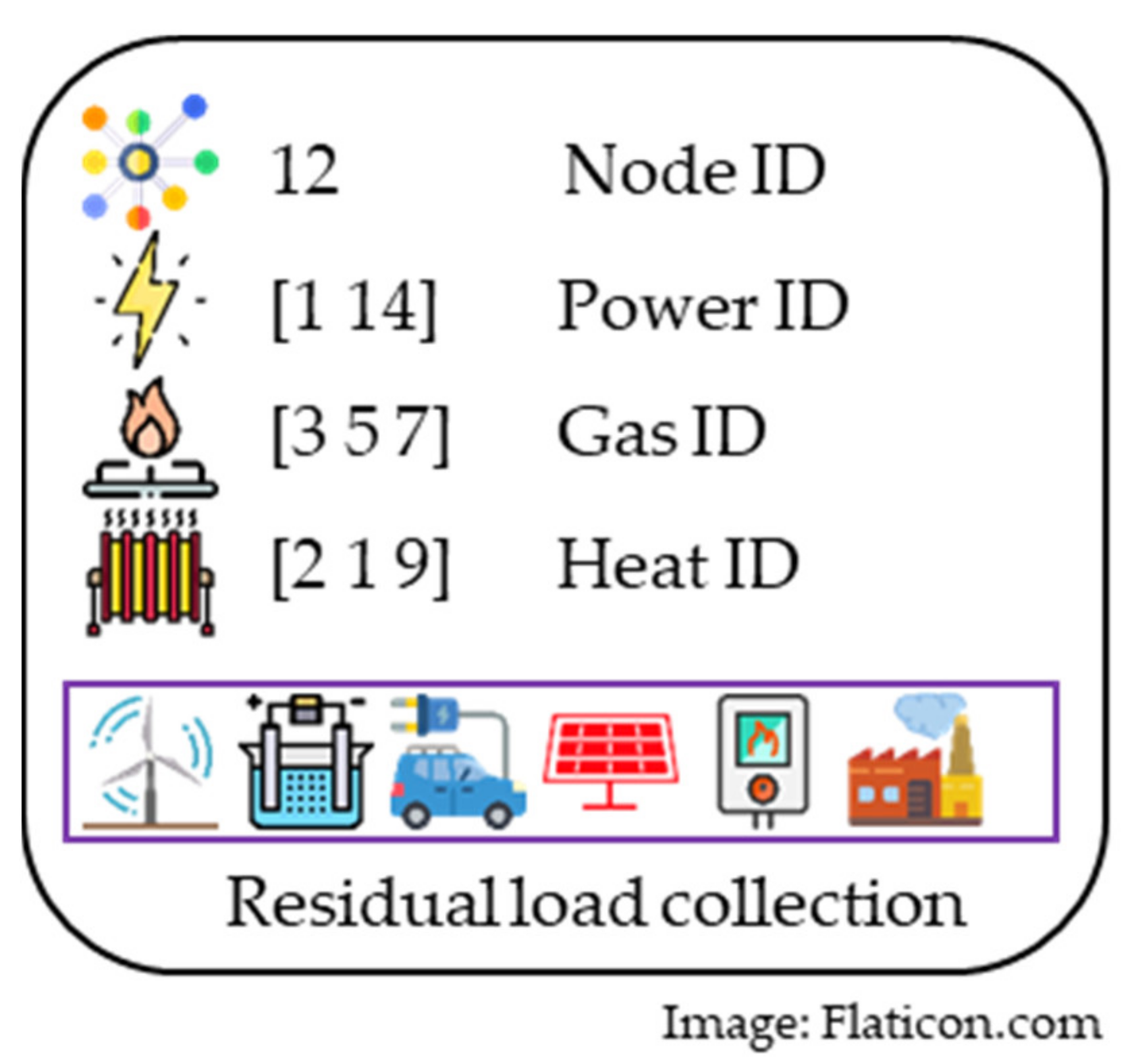
| Parameter | Type | Description |
|---|---|---|
| Node ID | scalar | One unique number is assigned to each node. |
| Power ID | 1 by 2 vector | Vector at [1 1] is currently a spare parameter. Vector at [1 2] indicates the node’s position in the power grid. |
| Gas ID | 1 by 3 vector | Vector at [1 1] indicates the node’s pressure level (e.g., 2 = 70 bar). Vector at [1 2] indicates the node’s subgroup. Vector at [1 3] indicates the node’s number within the subgroup. |
| Heat ID | 1 by 3 vector | Please refer to Gas ID. |
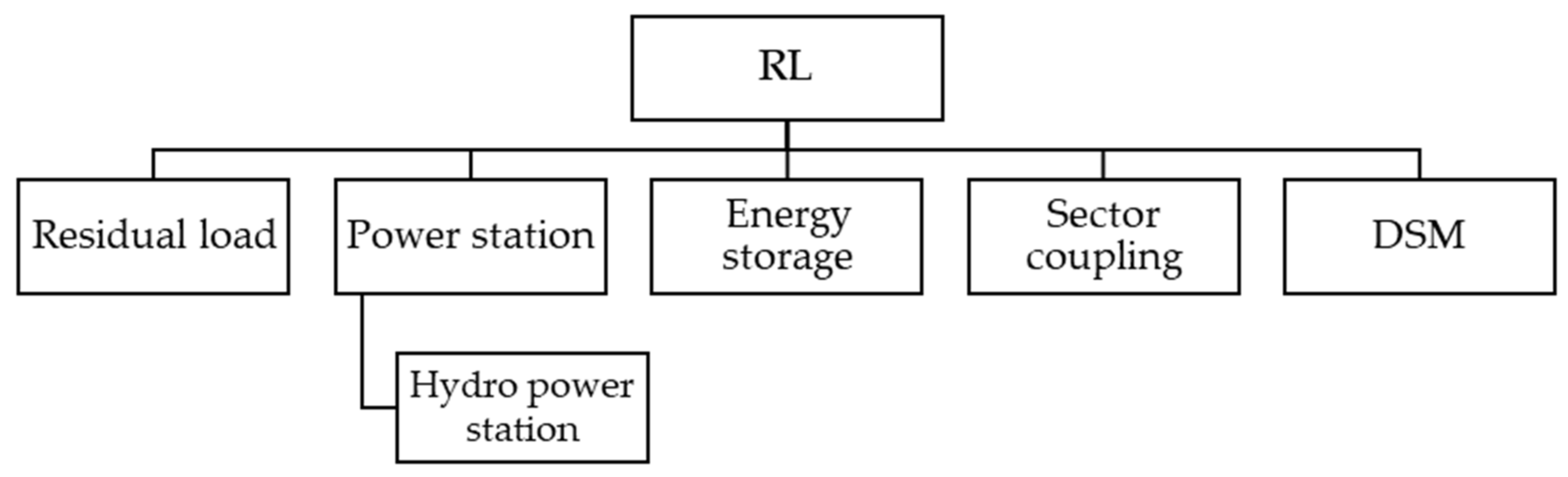
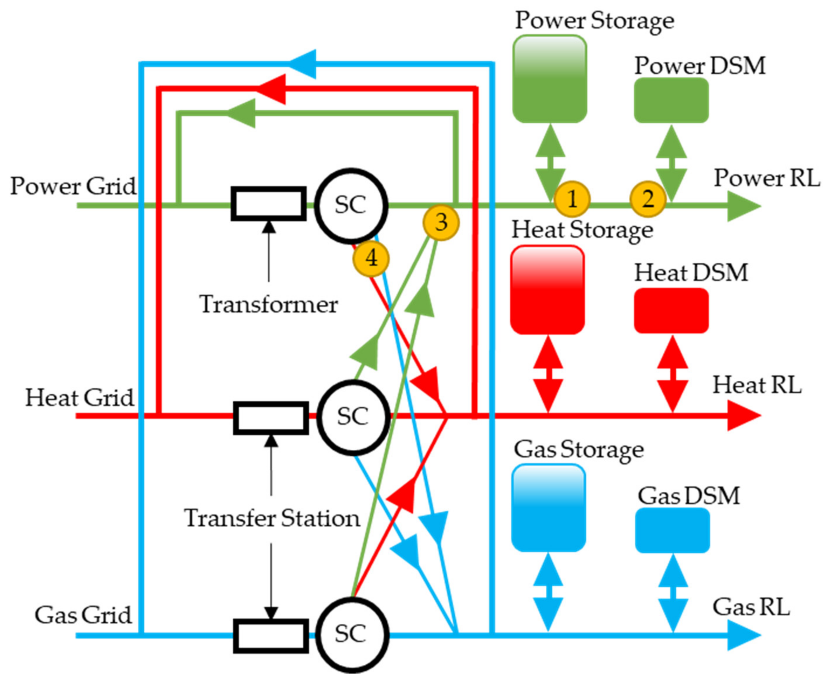
| RL collection | array | This array contains all objects, and their behavior can be expressed in active and reactive power, gas, or heat RL. Power RL is defined as per Equation (1), valid for all other energy carriers too. The RL collection in Figure 2 includes wind energy, electrolysis, electric car, photovoltaics, gas to heat (GtH), and an industrial consumer. |
| Parameter | Description |
|---|---|
| type | Defines the type of underlying object. Residual load or Power station 1: Pre-defined residual load profile or power station with predefined temporally resolved profiles (e.g., residual load, water flowrate). Sector coupling 2: Power to gas and heat (PtGH). 3: Power to heat (PtH). 4: Heat to power (HtP). 5: Gas to heat (GtH). 6: Gas to power and heat (GtPH). Energy storage 7: Power storage. 8: Gas storage. 9: Heat storage. DSM 10: Electric vehicle. 11: Demand-side management. |
| RLgas | This vector contains the object’s pre-set or calculated gas RL. The calculated gas RL depends on the object’s operating strategy. |
| RLheat | Refer to RLgas. |
| RLpower | Like RLgas, except that active and reactive power RLs are considered. |
| RLgasFlex | These parameters contain the object’s RL flexibility. The usage of these parameters depends on the object’s operating strategy. The implementation of flexibility is explained in Section 2.1.4. |
| RLheatFlex | |
| RLpowerFlex |
| RES | Generation 2018 | Expansion Until 2030 |
|---|---|---|
| Hydro | 37.6 TWh | +5 TWh |
| Wind | 6.0 TWh | +10 TWh |
| Photovoltaics | 1.5 TWh | +11 TWh |
| Biomass | 4.9 TWh | +1 TWh |
| Total | 50 TWh | +27 TWh |
| Scenario 1 | Scenario 2 | Scenario 3 | |
|---|---|---|---|
| Thermal generation and (pumped)-storage hydro | ENTSO-E | ENTSO-E | Flexibility |
| Electric vehicle | SLP | Optimized | Optimized |
| Battery storage | Greedy | Optimized | Optimized |
| Heat pump | Load following | Optimized with storage | Optimized with storage |
| Power grid calculation | PF | PF | OPF |
| Scenario 1 | Scenario 2 | Scenario 3 | |
|---|---|---|---|
| Overload time DG | 182,205 time steps | 206,592 time steps | 81,991 time steps |
| Average DG line overload | 38.8% | 42.5% | 35.5% |
| Count of overloaded DG lines | 39/480 | 57/480 | 40/480 |
| Overload time TG | 3904 time steps | 8131 time steps | 144 time steps |
| Average TG line overload | 16.0% | 16.3 | 30.1% |
| Count of overloaded TG lines | 5/104 | 7/104 | 6/104 |
| Scenario 1 | Scenario 2 | Scenario 3 | |
|---|---|---|---|
| Biomass | 6.0 TWh | 6.0 TWh | 6.0 TWh |
| Photovoltaics | 12.1 TWh | 12.1 TWh | 12.1 TWh |
| Wind | 15.5 TWh | 15.5 TWh | 15.5 TWh |
| Gas turbine and CHP | 10.8 TWh | 10.8 TWh | Consumption: 0.83 TWh Generation: 8.2 TWh |
| (Pumped)-storage hydropower | Consumption: 1.5 TWh Generation: 8.5 TWh | ||
| Hydropower>10 MW | 27.9 TWh | 27.9 TWh | 27.9 TWh |
| Hydropower≤10 MW | 11.6 TWh | 11.6 TWh | 11.6 TWh |
| Import | 8.1 TWh | 10.5 TWh | 3.7 TWh |
| Export | 36.0 TWh | 37.5 TWh | 23.0 TWh |
Publisher’s Note: MDPI stays neutral with regard to jurisdictional claims in published maps and institutional affiliations. |
© 2022 by the authors. Licensee MDPI, Basel, Switzerland. This article is an open access article distributed under the terms and conditions of the Creative Commons Attribution (CC BY) license (https://creativecommons.org/licenses/by/4.0/).
Share and Cite
Greiml, M.; Fritz, F.; Steinegger, J.; Schlömicher, T.; Wolf Williams, N.; Zaghi, N.; Kienberger, T. Modelling and Simulation/Optimization of Austria’s National Multi-Energy System with a High Degree of Spatial and Temporal Resolution. Energies 2022, 15, 3581. https://doi.org/10.3390/en15103581
Greiml M, Fritz F, Steinegger J, Schlömicher T, Wolf Williams N, Zaghi N, Kienberger T. Modelling and Simulation/Optimization of Austria’s National Multi-Energy System with a High Degree of Spatial and Temporal Resolution. Energies. 2022; 15(10):3581. https://doi.org/10.3390/en15103581
Chicago/Turabian StyleGreiml, Matthias, Florian Fritz, Josef Steinegger, Theresa Schlömicher, Nicholas Wolf Williams, Negar Zaghi, and Thomas Kienberger. 2022. "Modelling and Simulation/Optimization of Austria’s National Multi-Energy System with a High Degree of Spatial and Temporal Resolution" Energies 15, no. 10: 3581. https://doi.org/10.3390/en15103581