Article

The Impact of Urbanization on Land: A Biophysical-Based Assessment of Ecosystem Services Loss Supported by Remote Sensed Indicators

1
Italian Institute for Environmental Protection and Research (ISPRA), Via Vitaliano Brancati 48, I-00144 Rome, Italy
2
Department of Innovation in Biology, Agri-Food and Forestry Systems (DIBAF), University of Tuscia, Via San Camillo del Lellis SNC, I-01100 Viterbo, Italy
*
Author to whom correspondence should be addressed.
Land 2022, 11(2), 236; https://doi.org/10.3390/land11020236
Submission received: 3 December 2021 / Revised: 28 January 2022 / Accepted: 2 February 2022 / Published: 5 February 2022
(This article belongs to the Special Issue Dynamics of Urbanization and Ecosystem Services Provision)

Abstract

:
Urbanization and related land consumption are one of the main causes of ecosystem services loss. This is especially the case for soil-related services affecting ecosystem functions and limiting accessibility to natural resources. Satellite remote sensing and environmental databases enable in-depth analysis of urban expansion and land changes, which can be used to monitor trends in the provision of ecosystem services. This work aims to describe a multilayered approach to the assessment of biophysical loss of ecosystem services flows in Italy caused by an increase in land consumption in the period 2012–2020. The results show higher losses in wood production, carbon storage, hydrological regime regulation, and pollination in the northern regions of Italy, as well as in some southern regions, such as Campania and Apulia. Habitat quality loss is widespread throughout Italy, whereas crop production loss varies on the basis of the locations in which it occurs and the crop types involved. Loss of arable land and fodder production mainly occurs in northern regions, whereas southern regions have experienced a drop in permanent crop production. This study highlights the importance of using integrated data and methodologies for well-founded approaches, with a view to gaining a thorough understanding of ecosystem services-related processes and the changes connected therewith.

1. Introduction

Compact and dispersed patterns of urban expansion [1,2] are a global phenomenon and are one of the most important factors in landscape change [3,4]. Starting from the 20th century, the increasing demand for land to be used for buildings and infrastructures led to greater urbanization of previously natural and agricultural areas [5], making urbanization a major cause of land consumption. More generally, land consumption can be considered to be the change from non-artificial land cover to artificial land cover, with a distinction having to be made between permanent consumption (due to permanent artificial land cover, such as concrete or asphalt) and non-permanent consumption (due to reversible artificial land cover or soil alteration processes, such as, soil compaction in construction sites or excavations in quarries) [6,7]. The process of urbanization, and the related increase in impervious surfaces, affects other types of land use and land cover [8], triggering a series of effects on the environment, which results in it being the main cause of land degradation [9]. The main effects consist of the loss of fertile soils [10], the adverse impact on water balance [11], the increase in surface water runoff and flood risk [12], the negative influence on local microclimates due to urban heat islands [13,14], landscape fragmentation, and the loss of biodiversity [15,16]. Such effects limit the accessibility to natural resources and the provision of ecosystem services (ES), defined as the goods and benefits that people derive from ecosystems [17,18]. ES provision is a dynamic process and can be measured, in terms of flow, as the annual potential number of services provided by ecosystems [19,20].
Recent studies have focused mainly on drivers of change and the impact thereof on ES as a relevant issue to be understood, as well as the related implications on ecosystems functions and conservation [21], also including soil functions. Soils play a crucial role in providing several so-called soil ES [22,23], in particular provisioning and regulation services [24,25], contributing for example to food and wood production, hydrological flow regulation, carbon sequestration, pollination, habitat function, and biodiversity conservation [26]. Indeed, there is, through soil functions, a direct link of soil properties to specific ES, as indicated in Adhicari et al. [27]. In recent decades, policies and strategies have highlighted the importance of ES in maintaining livelihoods, and have stressed the fact that, for the purpose of providing ES, the natural land and agricultural system depend on soil. This is also confirmed by the recent EU Soil Strategy for 2030 [28], the EU Biodiversity Strategy for 2030 [29], and the Common Agricultural Policy [30]. The increasing amount of attention that is, with a view to fostering sustainable land development, paid at the international level to ecosystems, and the need to consider how changes in ecosystems affect human well-being [17,31,32], have given rise to an assessment being made both at a global level—based on the Aichi Biodiversity Targets [33] and the 2030 Agenda [34]—and at a European level [35]. The concept of ES, and the related frameworks that have been developed in connection therewith, have been recognized as being vital for supporting territorial management policies [17,22,36]. The various initiatives aim to improve the mapping of ecosystems, become apprised of the functional interactions and the pressures to which they are subjected, as well as establish indicators that assess changes in the provision of ES, in terms of the biophysical and economic aspects thereof [37].
ES assessment is a complex process, which involves integrating different scientific fields and several databases that vary in accuracy, scale, updating, and availability. Therefore, an approach based on various thematic layers is required, so as to have an overview of ES loss that supports the resource management decision-making process. Furthermore, monitoring land use and land cover spatial distribution, especially in urban areas, is essential for providing accurate and timely information to be used as input data that allows soil-based ES provision changes to be assessed. Within this context, major advances in satellite remote sensing have improved data collection and analysis methodologies used for the purpose of detecting artificial land covers [38,39,40,41]. These include the Sentinel satellite constellations of the EU Copernicus Programme [42] which provide high-resolution (spatial, spectral, and temporal) multispectral and SAR images suitable for measuring land consumption in a detailed manner [6].
In Italy, where land degradation processes due to land consumption are increasing, especially in agricultural and peri-urban areas [43], the Italian Institute for Environmental Protection and Research (ISPRA) is in charge of a monitoring program at the national level regarding: (i) land consumption mapping, based on a Sentinel satellite images analysis that is integrated with the photointerpretation of national orthophotos; (ii) land cover mapping, based on the integration of the Copernicus Land Monitoring Services (CLMS) datasets (Corine Land Cover, High Resolution Layers, Urban Atlas, Riparian Zones, and Natura 2000) and the national land consumption map; (iii) estimate of land degradation and ES changes (biophysical and economic) caused by annual land consumption. This study is the first work that is focused on Italy and that, in trying to collect and harmonize existing data, analyzes nationwide soil-based ES loss with a detailed spatial resolution. The paper aims to describe the multilayered approach that has been adopted in assessing biophysical loss of ES flows caused by land consumption increase in the period 2012–2020, as recorded by the aforementioned national monitoring program.
After having introduced the topic of ES and ES losses due to urban expansion, we describe the procedure adopted for the purpose of assessing changes in six ES in the period under examination. We describe the input data used and the methodologies applied for the purpose of analyzing the reference data and the additional thematic layers. The section in which the results are set out shows what losses were recorded for each ES. We then discuss the results of the analysis and considering the procedure’s achievements and shortcomings. Finally, we summarize the conclusions derived therefrom.

2. Materials and Methods
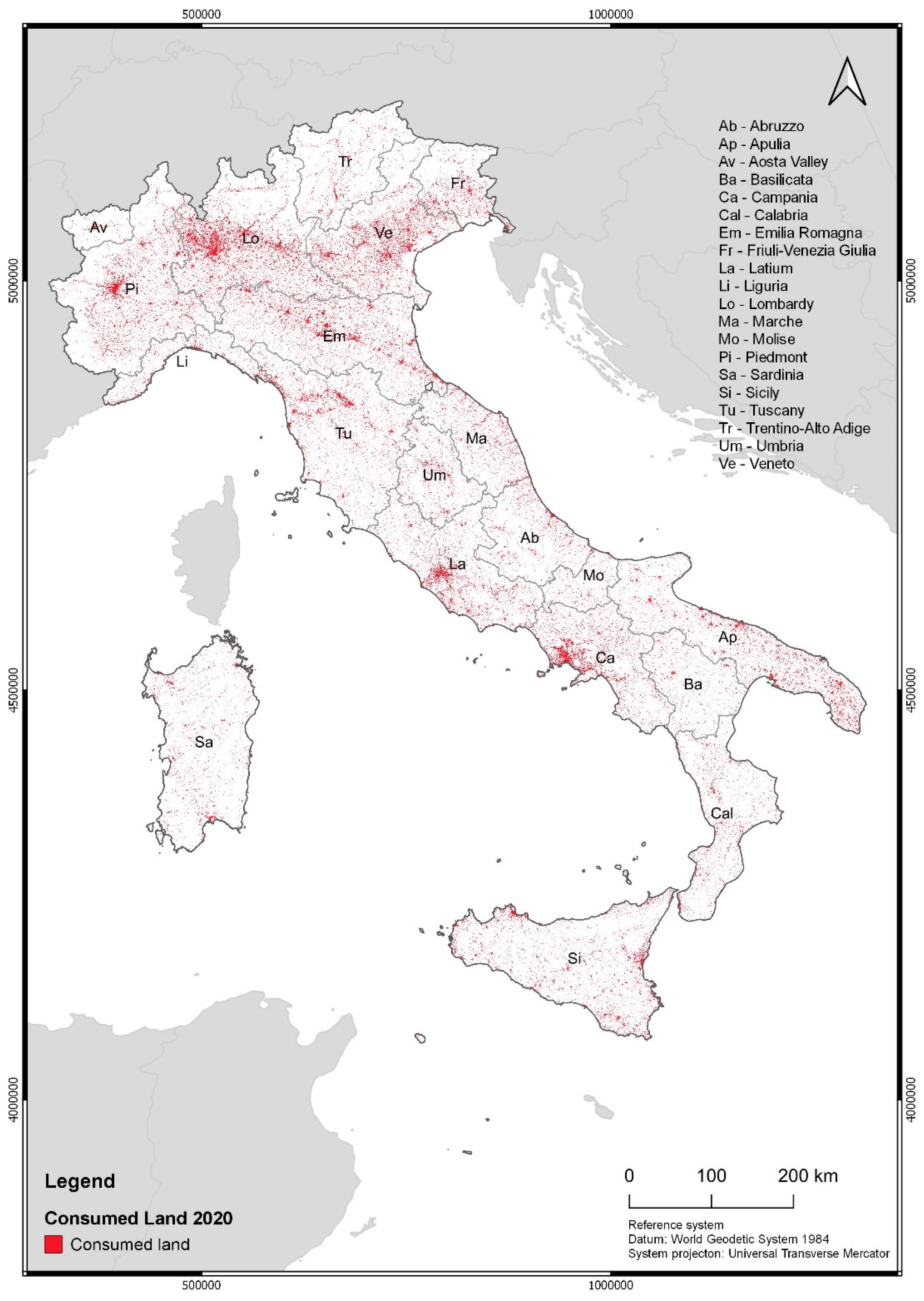
2.1. Study Area

Italy is located in the Mediterranean basin (southern Europe), it covers around 300,000 km2 and is divided into 20 administrative regions. It is a peninsula characterized by two mountain ranges (the Alps and the Apennines), wide river valleys, two major islands (Sardinia and Sicily), and various other small islands. Italy’s physiography and geographical position have led to it having heterogeneous features in terms of climate (ranging from a Mediterranean climate along the coastline to an alpine climate at the higher elevations) and in terms of land use/land cover, with urban areas concentrated in the plains and along the coasts, which cover 7.1% of the national territory (year 2020) (Figure 1 and Figure 2) [44].

2.2. Reference Data

The basic cartographic maps used to detect changes in the provision of ES in Italy are the national land cover map and the national land consumption map. These maps are the common data source for all the ES analyzed in this study.
The national land cover map is based on the integration of the Copernicus Land Monitoring Services (CLMS) datasets (namely the Corine Land Cover, High Resolution Layers, Urban Atlas, Riparian Zones, and Natura 2000 datasets). The datasets show differences in the classification systems, resolutions, and updating frequencies adopted. Therefore, a harmonization procedure had to be adopted in order to make the datasets comparable. De Fioravante et al. [45] followed the EIONET EAGLE (Action Group on Land monitoring in Europe) group framework, which provides a methodology for describing land cover and land use data in a consistent manner. The CLMS data were integrated in an EAGLE compliant land cover map for the year 2012 (10 m resolution), which includes 16 classes of land cover (Figure 1).
The national land consumption map is, on the other hand, a product generated by the processing of Sentinel-1 (based on the SAR backscatter of VH polarization threshold) and Sentinel-2 (based on Normalized Difference Vegetation Index extraction and threshold value) satellite images, and photointerpretation of national orthophotos. The land consumption map is updated every year with a spatial resolution of 10 m [6,44]. National land consumption maps for the years 2012 and 2020 (Figure 2) were used for the purpose of assessing ES changes.
Land consumption is mapped both in its permanent and temporary forms following the definition given by [6,7]. By permanent consumed land, artificial surfaces composed of impervious material (e.g., concrete, asphalt or tarmacadam), both 3D (buildings) and 2D (roads), were taken into consideration (6.6% of the Italian national territory). This component is assumed to be irreversible, since extremely long amounts of time are required for restoring soil to its the natural state. Reversible consumed land is the result of compaction in construction sites, excavations in quarries, temporary coverage with artificial surfaces and other forms of soil alteration that do not imply permanent consumption, but that adversely affect the soil’s natural state. However, this component is a minor (albeit dynamic) part of the total consumed land (0.5% of the Italian national territory). In light of the limited extent thereof and taking into account that for some portions of Italy’s territory the distinction between permanent and temporary forms of land consumption is lacking, both components are considered as consumed land, without any exception whatsoever (Figure 2). Figure 3 shows some examples of land consumption in urban, agricultural, and natural environments in the period under investigation.

2.3. Biophysical Assessment of Loss of Ecosystem Services Flows

The biophysical evaluation of Italy’s territory concerned six ES: crop production, carbon storage, wood production, habitat quality, hydrological regime regulation, and pollination. The land cover and land consumption maps were used as data input for all six ES, and other appropriate data inputs were added for each ES. Specific methodologies or already existing analysis models were adopted for each ES, taking into consideration the loss of ES flow in light of the reduction in the current yearly potential provision thereof, due to the increase in land consumption. Consumed land leads to soil-based ES being reduced to zero, since the soil no longer performs its functions. The analyses were conducted at the national and regional level and were performed using QGIS 3.20 [46] and InVEST 3.9.1 (Integrated Valuation of Ecosystem Services and Tradeoffs) [47] software.

2.3.1. Crop Production

Crop production is essential for food supply. Land take due to urbanization nullifies the land’s capacity to cultivate and produce the resulting goods and benefits. With a view to estimating the provisioning of crop production, and the loss of flow in the period under examination due to land consumption increase, data on surface cover (hectares) and production (quintals) for each crop types were, in respect of each Italian administrative province, taken from the national census of agriculture carried out by the Italian National Institute of Statistics (ISTAT) (year 2013) [48]. The crop types were grouped into five classes (fruit trees, olive groves, vineyards, fodder, and arable land). Data on crop production were then spatialized for the purpose of obtaining the values in q/ha, and then in q/pixel compliant with the land cover and land consumption maps’ spatial resolution. The amount of crop production in 2012 and the potential loss in the period from 2012 to 2020 on account of land consumption were calculated. Even though the quintal is not considered in the International System of Units, it is widely used, especially in Europe, and it is the unit of measurement with which data are officially released by ISTAT. For these reasons, the results of changes in agricultural production will be presented in quintals (1 q = 100 kg).

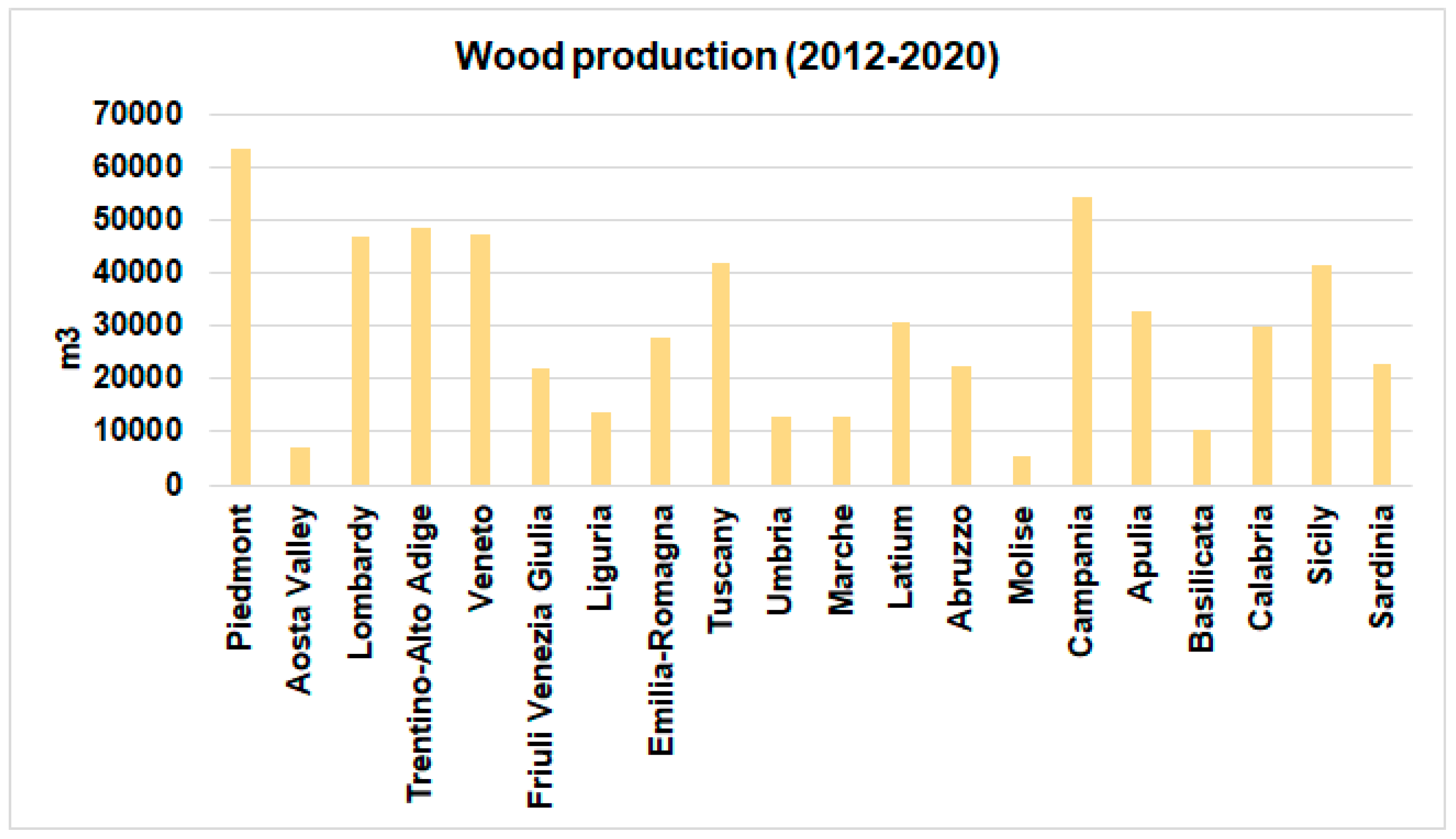
2.3.2. Wood Production

The production of wood raw materials is a provisioning service supplied to a large extent by natural forest and tree plantations. As is the case with crop production, the urbanization of areas covered by forests leads to wood production ES flow being completely lost. The method adopted follows the For-est model [49,50] concerning the above ground biomass, which uses the National Inventory of Forests and Forest Carbon Tanks (INFC) data (classified by administrative region and forest typology) [51] as input data. The model takes into consideration four main forest management categories: stands, coppices, plantations, and protective forests. It uses, through the Richards function [49], growing stock as the only driver for the purpose of estimating the evolution of forest carbon pools (above ground and below ground biomass, dead wood and litter, and soil organic matter) over time. The lack of detailed, homogenous and georeferenced data for all of the arboricultural systems in Italy has led to the simplification of the national methodology. The average annual index of the above ground biomass volume increase, which is calculated by the For-est model and utilizes the historical series of INFC data, is used to assess the biophysical value of the ES flow. All of the land cover map’s forest classes were, therefore, considered in the same way and the same average annual index was applied to them. The change from forest area to consumed land resulted in this index being reduced to zero.

2.3.3. Carbon Storage

Carbon storage is a regulation service provided by terrestrial and marine ecosystems thanks to their ability to fix greenhouse gases [52]. This service contributes to the regulation of the climate at a global level and plays a fundamental role in the context of climate change mitigation and adaptation strategies. The model Carbon Storage and Sequestration of InVEST software was used to assess the carbon storage loss using the INFC and the National Soil Organic Carbon Map [53] as a data source. The land cover classes were associated with the INFC forest typologies [54]. Four different carbon pools, according to the Intergovernmental Panel on Climate Change classification [55], were taken into consideration for each land cover type: above ground biomass, below ground biomass, dead organic matter, and soil organic matter. Specific coefficients were used for the purpose of identifying different pools’ contribution thereto [56,57,58].
The flow of carbon content regarding above ground and below ground biomass volume for forest types and permanent crops is expressed as a function of the growth rate taking as a reference point the growing stock data provided by the INFC for each forest type, and Caneveira et al. [59] for permanent crops. In [59], the authors proposed default carbon stock values for olive trees, vineyards, and fruit trees in which the age of plantations is known (1, 5, 10, 15, and 20 years). The average increase for these crop types is given by the difference between the value of 20 years and that of 5 years divided by the 15 years that elapse. Literature values were used for other natural and agricultural areas [60], and artificial areas are considered as zero. With regard to the carbon contained in the dead organic substance, the necromass values are deduced from those of the above ground biomass through coefficients (0.20 for evergreen plants and 0.14 for deciduous trees, source [55]), whereas those in the litter specific formulas for each species reported in the bibliography were used [56,61]. As far as the soil organic pool is concerned, the values reported in the National Soil Organic Carbon Map were used. The map contains the values of the carbon contained in the soil up to a depth of 30 cm, in raster format and with a resolution of 1 km. See [45] for a detailed description of carbon storage ES assessment.

2.3.4. Habitat Quality

This is a regulation service which, in supplying different types of habitats, contributes to human well-being by guaranteeing ecosystem functionality, biodiversity maintenance, and environmental resilience. Various anthropogenic factors have an impact on habitat quality, causing degradation and alteration of ecological processes [62]. With a view to assessing the loss of ES flow due to land consumption in the period under investigation, the Habitat Quality model of the InVEST software has been used. In this model, habitat quality is assessed in relation to different land use and land cover classes [47], on the basis of the premise that areas with higher habitat quality host a greater number of species and that habitat size and quality decrease lead to a decline in the persistence of species [63]. After having associated the land cover classes with habitat types (according to the EUNIS classification [64]), a habitat suitability value for each land cover class, for the purpose of assessing its ability to provide a habitat for biodiversity, has been assessed, ranging from 0 to 1, where 1 indicates habitat with the highest suitability for species biodiversity [65]. Three types of threats affecting habitat suitability have been taken into account: the habitat’s sensitivity to being influenced by different types of threats, the impact (weight) of different threats on each habitat type, and the maximum distance at which the threats can affect the habitat. A threats impact value has been assessed, ranging from 0 (absence of threat) to 1 (presence of threat). The habitat suitability values and the threats parameters, which have been used as input data in the InVEST model, have been set through an expert-based approach [66] (Table 1 and Table 2), using a questionnaire put to over 41 national experts, whose results are described in [67]. The result is a map of habitat quality in which the cell values range from 0 to 1, where 1 indicates high habitat quality. The ES was estimated ranking the range in five classes (class 1 poor habitat quality, class 5 high habitat quality) and assessing the surface variation in the period 2012–2020 for each class.

2.3.5. Hydrological Regime Regulation

With regard to regulation services, hydrological regime regulation is an important water cycle-related ES. The evaluation thereof is based on the BigBang 1.0 (Nationwide GIS-based hydrological water budget on a regular grid) hydrological model developed by ISPRA for the purpose of evaluating the factors of hydrological balance at national level, with a GIS-based spatially distributed procedure being used that assesses the water budget components at different spatial and temporal scales [68]. Total precipitation, actual evapotranspiration, surface runoff, and groundwater recharge are evaluated on a monthly basis directly on the grid with a 1 km resolution. The procedure allows the effects produced by soil consumption increase in the period 2012–2020, in terms of increase in surface runoff, to be verified. This is done by applying the land cover and the land consumption maps, while the climatic conditions are considered as values mediated over the period in question. In this paper, the BigBang 1.0 version has been used. A BigBang 4.0 version has, however, recently been released for national accounting purposes [69] and will be tested for future improvements in ES assessment.

2.3.6. Pollination

Pollination is an important regulation service for agriculture production and ecosystems well-being [70,71] which is threatened by urbanization, agriculture intensification, and the use of pesticide and fertilizers [72,73]. The provision of this ES depends on the availability of nesting habitats and floral resources, and on the foraging distance of pollinators [74]. The InVEST Crop Pollination model was used to evaluate this ES. 50 species of pollinators (bees and bumblebees) were selected for the Italian national territory [75] (Table 3), and their characteristics were associated with the land cover classes and then analyzed, in terms of the availability of hosting pollinating species according to the types of nesting (reeds, rocks, cliffs, walls, plant stems, soil, and dead wood). The Italian national territory was divided on the basis of the altitude range (less than 800 m, from 800 to 1600 m, from 1600 to 2100 m, and over 2100 m) and the three main biogeographical regions (Mediterranean, Continental and Alpine), taking into account each of the resulting areas’ different vegetation and different pollen production periods. In particular, the information used were: the type of nesting, period of activity, maximum flight distance, preferences among the varieties of nests, presence of flowers, and pollen period for the most widespread plants. The abundance of pollinators in each area were, therefore, considered as a “source” and subsequently the distribution on the agricultural surfaces to be pollinated were estimated (i.e., the potential index of abundance of pollinators that can reach an agricultural area). The result is a map in which the availability of pollinators for a potential agricultural area to be pollinated is estimated and the cell values range from 0 (low availability) to 1 (high availability). The ES flow was estimated, ranking the range in four classes (class 1 poor pollination, class 4 high pollination) and assessing the surface variation in each class in the period under investigation.

3. Results

3.1. Crop Production Loss

In 2012, agricultural production in Italy amounted to 915,705,580 quintals (q), with an average production of 45,785,279 q. Looking in detail at regional production (Figure 4), fruit trees had their highest production in Sicily and Calabria (12,861,590 q and 9,909,800 q, respectively), whereas production was below 7 q in the other regions. The region with the highest production levels for olive groves was Apulia, with 8,213,754 q, whereas the highest production level for vineyards was recorded in Apulia and Sicily (around 15,000,000 q) and in Veneto with 8,099,192 q. As far as fodder is concerned, the highest production level was recorded in Lombardy (32,761,977 q) and Emilia-Romagna (26,786,595 q), whereas it remained below 15,000,000 q in the other regions. Emilia-Romagna also recorded the highest production level for arable crop production (107,583,166), followed by Lombardy, Veneto, Piedmont, and Apulia, with around 50,000,000 q.
In Italy, a loss of approximately 4,154,559 q of agricultural products due to land consumption in the period 2012–2020 was estimated (0.45% of percentage loss). The greatest drop occurred in the class of arable land (2,533,940 q, 0.43%), followed by fodder, fruit trees, vineyards, and olive groves, with a loss of approximately 974,403 (0.56%), 307,691 (0.45%), 247,670 (0.41%), and 90,853 q (0.42%) in the products generated therefrom, respectively (Table 4). At the regional level (Figure 5, Table 4), Emilia-Romagna is the region that has the highest variation in arable land production (376,972 q, 0.35%), followed by Veneto (372,463 q, 0.72%), and Lombardy (270,171 q, 0.50%). In the other regions, the loss is between 50,000 and 100,000 q and it is less than 50,000 q in only five regions, with the lowest value being recorded in the Aosta Valley, where the loss was approximately 3,536 q, which corresponded to a loss of 0.90%. As far as the fodder category is concerned, the greatest loss occurred in Lombardy (approximately 250,000 q, 0.76%), followed by Campania (130,000 q, 0.64%), Veneto (131,000 q, 0.75%), Trentino-Alto Adige, Emilia-Romagna, and Latium (79,000, 87,000 and 86,500 q, respectively), corresponding to a 0.60% loss in the regional fodder production in Latium and Trentino-Alto Adige, and 0.35% in Emilia-Romagna. In the other regions, the loss was less than 20,000 quintals, with the exception of Piedmont (around 42,000 q). The lost production of olive groves caused by land consumption was greater in Apulia, with a drop of 50,000 q (0.60%), whereas it was less than 10,000 q in the other regions. As far as the fruit trees category is concerned, Calabria and Sicily lost almost 40,000 (0.41%) and 75,000 q (0.58%), Trentino-Alto Adige 39,000 q (0.76%), and Campania and Apulia 30,000 q (0.65% and 0.49%, respectively). On the other hand, the loss was lower (below 10,000 q) in the other regions. Finally, the variation in vineyards due to soil consumption in the period under examination led to a reduction of about 10,000 q in all of the regions, with the exception of Apulia (58,200 q, 0.38%), Sicily (60,160 q, 0.40%), and Veneto (56,000 q, 0.69%).

3.2. Wood Production Loss

At the national level, a total loss of 595,063 m3 of wood production was estimated. At the regional level, Piedmont is the region with the highest loss (63,520 m3), followed by Trentino-Alto Adige, Veneto, Lombardy, and Campania with a loss of around 50,000 m3. In the other regions, the loss of flow is between 10,000 and 50,000 m3, apart from Molise and the Aosta Valley, which have the lowest values (5,628 and 6.963 m3 respectively) (Figure 6).

3.3. Carbon Storage Loss

In Italy, a loss of about 17,000 tons of stored carbon due to land consumption was estimated between 2012 and 2020. At the regional level, the greatest loss occurred in Piedmont, Trentino-Alto Adige, and Veneto (1902, 1731, and 1686 tons, respectively), with a considerable contribution also being provided by the Lombardy, Campania, and Sicily regions (between 1200 and 1500 tons). Values below 250 tons were estimated for the Marche, Umbria, Basilicata, Molise, and Aosta Valley regions (Figure 7).

3.4. Habitat Quality Loss

Figure 8 shows the surface variations of ES flow at the regional level for each class of habitat quality. Class 1 (poor quality) records an increase of above 1% for all of the regions (between 1% and 3%), with the highest percentages being recorded for the Trentino-Alto Adige, and Abruzzo regions. Classes 2 and 3 record a slight decrease, with only Veneto and Apulia reaching 1% for class 2 and class 3, respectively. Class 4 has not recorded considerable changes, with the exception of Trentino-Alto Adige and the Aosta Valley, where increases of 2% and 1.4%, respectively, have been recorded. Class 5 has recorded a slight decrease, with the greatest changes being recorded for Sicily, Trentino-Alto Adige, and Campania (0.5–0.6%).

3.5. Hydrological Regime Regulation Loss

An estimate was made, in the period 2012–2020, of the impact that the increase in land consumption had on surface runoff (which represents the hydrological regime regulation service). Figure 9 shows the variations in hm3 in this service caused by the consumption of land in Italy. At the national level, an increase of about 250 hm3 of surface runoff was estimated. The biggest increases were recorded in the Veneto and Lombardy regions (50 and 44 hm3, respectively), whereas the smallest increases (less than 10 hm3) were recorded in the Umbria, Basilicata, Liguria, Molise, and Aosta Valley regions.

3.6. Pollination Loss

Figure 10 shows the surface variations of ES flow at the regional level for each class of pollination. Class 1 (poor pollination) records a slight increase, with the highest value being recorded for Apulia (0.7%). Class 2 records an increase in almost all regions, with the highest percentages to be found in Trentino-Alto Adige and Campania (0.9%). Classes 3 and 4 record a decrease in all regions and the greater variations have been estimated in Veneto, Friuli-Venezia Giulia, Lombardy, Campania, and Marche (between −1% and −3%) for class 3, and the Aosta Valley and Trentino-Alto Adige (−3.4% and −1.6%, respectively) for class 4.

4. Discussions

This study has assessed, from a biophysical point of view and with a multilayered approach, the changes occurring in the provision of ES flows as a result of land consumption in Italy This has made it possible to integrate and harmonize the large amount of heterogeneous data available in Italy so as to better interpret the ongoing land dynamics and how these affect the availability of goods and services offered by ecosystems. The results have explained how transformations have occurred in Italy over the selected time interval, which have mainly been driven by urbanization. The loss of crop production varies in Italy, depending on the type of crops involved. Loss of arable land and fodder production mainly affects the northern regions, whereas southern regions show a decrease in permanent crop production. Even if the percentage variations in crop production are low, they are nevertheless important because, in many cases, agricultural areas are based on important biological and cultural practices that are difficult to replace [76], and they also play a role in carbon storage and pollination assessment. Wood production and carbon storage losses affect the northern regions more, as well as the Campania region. The northern regions also show an increase in water runoff, with potential consequences for the hydrological regime regulation service. As far as habitat quality is concerned, the increase in the lowest quality class is widespread throughout Italy. The northern regions and the Campania region have recorded a drop in pollination ES availability. Since urban expansion is a process affecting more the lowlands, the higher losses in ES flows have mainly been recorded in the northern regions which include the Po plain, and the plains of Campania and Apulia in the south. These findings are in line with the demographic dynamics model of wealthier countries proposed since the late 1980s [77]. Indeed, whereas compact urban growth has been frequently associated with population increase and economic development, which is typical of most of the European countries after World War II [5], the advanced economies have been characterized in the last decades by the outward expansion of low-density settlements [78,79], often occurring in fertile agricultural areas [9,80]. Other research studies dealing with the impact of urbanization on ES have confirmed losses of stored carbon, agricultural production, habitat quality, and flood mitigation in developing urban areas [25,81,82], also leading to land reclamation and deforestation in rural areas [82].
The accurate localization of these processes has benefited from the detailed information provided by the input data. The high resolution of Sentinel satellites images and CLMS datasets and their high frequency availability enable an in-depth analysis of land consumption changes consistent with the EU requests and useful for the purpose of monitoring trends in ES provisions and flows to be conducted. The outcomes show that the proposed approach is effective in giving an overall assessment of the ES by using spatially explicit data and models. Indeed, these products of the monitoring program are already gathered in the national Environmental Data Yearbook [83], which is the official collection of nationwide data and information concerning the environment in Italy. Furthermore, they are used for national environmental monitoring policies, such as the National Capital Accounting [84], and could be a point of reference for the implementation of the various environmental policies, first of all the EU Soil Strategy for 2030 [28], in which the important role played by ES in maintaining ecosystems and human well-being is highlighted.
However, there is still room for improvement, especially with regard to models and input data. The need for more detailed information has arisen. For example, the inappropriate use of conventional agriculture technology and improper forest management practices can have negative short-term effects on crop and wood production, but can also have adverse effects on other ES in the long term. As a result thereof, a national evaluation of biophysical loss of ES must be integrated with more detailed information, for example on agricultural practices, forest management practices, and water balance at river basin level. A further example to be found in this study concerns the wood production analysis. An up-to-date database that localized arboriculture plants, forest types, age, provision, and forms of management would be needed for the purpose of developing a methodology able to overcome the simplification and achieve better results.
Furthermore, one of the main shortcomings arising therefrom concerns the data updating frequency. While the national land cover and land consumption maps are generated by analyzing datasets, satellite images, and remote-sensed indicators obtained from the Copernicus program, which guarantee a frequent data updating that is compliant with the requirements of the national monitoring program, other data concerning thematic issues required for conducting a biophysical assessment of the ES selected in this study are provided less promptly and are updated less regularly. These differences confirm the need, with a view to having more accurate and reliable results, for improved national spatial data that enhance spatial and temporal dynamics evaluations in the provision of goods and benefits. A data release agreement that is more suitable for a monitoring plan should be considered, on account of the replicability of the methodology that can only be guaranteed by satellite and spatial data being available on a regular basis. This is an important issue to take into consideration to make the analysis of soil-based ES a consolidated procedure for the purpose of increasing the effectiveness of sustainable spatial planning. ES spatial distribution and evolution over time is, indeed, able to gather and aggregate complex information [85] that can be used by decision-makers as a tool for land sustainability evaluation [86] that encourages development with less ES degradation [87].

5. Conclusions

This study is the result of a first attempt to present an assessment of nationwide biophysical loss ES flows caused by land consumption as an indicator of urbanization in Italy at a detailed spatial resolution, dealing with the problem of the lack of accurate and available information for the whole study area, and trying to collect and harmonize existing data from different scientific fields. Indeed, the concept of ES, and the related frameworks developed at the international level, have been recognized as fundamental for supporting territorial management policies, and the importance of biophysical quantifications has been emphasized, with a view to supporting economic evaluations and natural capital management. The multitemporal analysis set out herein may serve as a tool for stakeholders and policymakers that allows them to understand the impact of human activities, and in particular urbanization, on land cover pattern, the rates of variation, and the causes that give rise to changes in the provision of ES. Furthermore, remote sensing and GIS technologies make it possible to analyze, assess, and map ES at different spatial and temporal scales for the purpose of understanding how the provision thereof varies according to territorial dynamics and different underlying socioeconomic circumstances, and how the synergies and trade-offs between the various ES in certain landscapes occur.
The evaluation of soil-based ES is becoming increasingly important in the context of land planning, since urban planning predominantly has an impact on soil resources. The six ES investigated herein are strictly connected with soil properties and functions, and modifications of this resource on account of urban expansion can affect the ecosystems’ ability to provide goods and benefits. Therefore, soil-based ES are a valuable reference-point and provide useful indications to administrations for the purpose of sustainable development policies and land planning, both at the national and local scale, even though they have to date not yet found a stable and codified position in the land use planning process.
Moreover, our study underlines the importance of using multilayered thematic data and the detailed localization of rapid changes that support the investigation of how urbanization affects ES and provides suggestions for how urban planning can be conducted with a view to ES protection, sustainable urban development, and human well-being. For this reason, this paper has pointed out the importance of using integrated data and methodologies, as well as more consistent and detailed data inputs. This allows well-founded approaches to be adopted, with a view to gaining both a thorough understanding of ES-related processes and the changes therein that are taking place, as well as acquiring a reference framework for the purpose of also gaining further insights that evaluate ES at different scales, from national to local levels. Further developments and improvements in the methodology are foreseen, especially as far as the search for updated and accurate thematic data and the use of new analysis models is concerned. In this respect, the Horizon 2020 project (SERENA: Soil Ecosystem seRvices and soil threats modElling aNd mApping) is currently conducting an in-depth analysis of this approach at the European level, whereas the LIFE preparatory project (NewLife4Drylands: Remote sensing oriented nature based solutions towards a NEW LIFE FOR DRYLANDS) is doing so at the local level. The results generated therefrom may serve as a basis for tackling multiscale landscape management and planning issues.

Author Contributions

Conceptualization, F.A. and D.S.; Methodology, F.A., A.S. and M.M.; Formal analysis, A.C., L.C., C.G., N.R. and A.S.; Writing—original draft preparation, D.S.; Writing—review and editing, F.A., D.S., C.G., L.C., C.G., N.R., A.S. and M.M.; Supervision, F.A. and M.M. All authors have read and agreed to the published version of the manuscript.

Funding

This manuscript is not funded by a specific project grant.

Data Availability Statement

The data supporting the findings of this study are openly available at https://groupware.sinanet.isprambiente.it/uso-copertura-e-consumo-di-suolo/library/consumo-di-suolo.

Acknowledgments

The authors want to acknowledge the European Union’s Horizon 2020 research and Innovation programme that under the ongoing project SERENA (grant agreement No. 862695) will support further development of the methodology presented in this study at the European level. Moreover, the authors want to acknowledge the ongoing project NewLife4Drylands (LIFE20 PRE/IT/000007) that gives the opportunity to conduct an in-depth analysis of this approach at the local level.

Conflicts of Interest

The authors declare no conflict of interest.

References

  1. Bruegmann, R. Sprawl: A Compact History; University of Chicago Press: Chicago, IL, USA, 2005. [Google Scholar]
  2. Schneider, A.; Woodcock, C.E. Compact, dispersed, fragmented, extensive? A comparison of urban growth in 25 global cities using remotely sensed data, pattern metrics and census information. Urban Stud. 2008, 45, 659–692. [Google Scholar] [CrossRef]
  3. Elvidge, C.D.; Tuttle, B.T.; Sutton, P.C.; Baugh, K.E.; Howard, A.T.; Milesi, C.; Bhaduri, B.; Nemani, R. Global Distribution and Density of Constructed Impervious Surfaces. Sensors 2007, 7, 1962–1979. [Google Scholar] [CrossRef] [PubMed]
  4. Stathakis, D.; Perakis, K.; Savin, I. Efficient segmentation of urban areas by the VIBI. Int. J. Remote Sens. 2012, 33, 6361–6377. [Google Scholar] [CrossRef]
  5. Smiraglia, D.; Salvati, L.; Egidi, G.; Salvia, R.; Giménez-Morera, A.; Halbac-Cotoara-Zamfir, R. Toward a New Urban Cycle? A Closer Look to Sprawl, Demographic Transitions and the Environment in Europe. Land 2021, 10, 127. [Google Scholar] [CrossRef]
  6. Strollo, A.; Smiraglia, D.; Bruno, R.; Assennato, F.; Congedo, L.; De Fioravante, P.; Giuliani, C.; Marinosci, I.; Riitano, N.; Munafò, M. Land consumption in Italy. J. Maps 2020, 16, 113–123. [Google Scholar] [CrossRef]
  7. Riitano, N.; Dichicco, P.; De Fioravante, P.; Cavalli, A.; Falanga, V.; Giuliani, C.; Mariani, L.; Strollo, A.; Munafò, M. Land consumption in italian coastal area. Environ. Eng. Manag. J. 2020, 19, 1857–1868. [Google Scholar] [CrossRef]
  8. Grimm, N.B.; Faeth, S.H.; Golubiewski, N.E.; Redman, C.L.; Wu, J.; Bai, X.; Briggs, J.M. Global Change and the Ecology of Cities. Science 2008, 319, 756–760. [Google Scholar] [CrossRef] [PubMed] [Green Version]
  9. EC (European Commission). Guidelines on Best Practice to Limit, Mitigate or Compensate Soil Sealing. Available online: https://ec.europa.eu/environment/soil/pdf/guidelines/pub/soil_en.pdf (accessed on 17 October 2021).
  10. Ceccarelli, T.; Bajocco, S.; Perini, L.; Salvati, L. Urbanisation and Land Take of High Quality Agricultural Soils–Exploring Long-term Land Use Changes and Land Capability in Northern Italy. Int. J. Environ. Res. 2014, 8, 181–192. [Google Scholar] [CrossRef]
  11. Haase, D. Effects of urbanisation on the water balance–A long-term trajectory. Environ. Impact Assess. Rev. 2009, 29, 211–219. [Google Scholar] [CrossRef]
  12. Yang, B.; Li, M.-H. Ecological engineering in a new town development: Drainage design in The Woodlands, Texas. Ecol. Eng. 2010, 36, 1639–1650. [Google Scholar] [CrossRef] [Green Version]
  13. Shiguang, M.; Fei, C.; Qingchun, L.; Shuiyong, F. Impacts of Urban Processes and Urbanization on Summer Precipitation: A Case Study of Heavy Rainfall in Beijing on 1 Aug 2006. J. Appl. Meteorol. Climatol. 2011, 50, 806–825. [Google Scholar] [CrossRef]
  14. Zhou, X.; Wang, Y.-C. Dynamics of Land Surface Temperature in Response to Land-Use/Cover Change. Geogr. Res. 2011, 49, 23–36. [Google Scholar] [CrossRef]
  15. Collinge, S.K. Ecological consequences of habitat fragmentation: Implications for landscape architecture and planning. Landsc. Urban Plan. 1996, 36, 59–77. [Google Scholar] [CrossRef]
  16. Bennett, A.F.D.; Saunders, A. Habitat fragmentation and landscape change. In Conservation Biology for All; Sodhi, N.S., Ehrlich, P.R., Eds.; Oxford University Press: Oxford, UK, 2010. [Google Scholar] [CrossRef] [Green Version]
  17. MEA (Millennium Ecosystem Assessment). Ecosystems and Human Wellbeing: Synthesis; World Resource Institute: Washington, DC, USA, 2005. [Google Scholar]
  18. Haines-Young, R.H.; Potschin-Young, M.B. Common International Classification of Ecosystem Services (CICES) V5.1 and Guidance on the Application of the Revised Structure. Available online: www.cices.eu (accessed on 30 November 2021).
  19. Schröter, M.; Barton, D.N.; Remme, R.P.; Hein, L. Accounting for capacity and flow of ecosystem services: A conceptual model and a case study for Telemark, Norway. Ecol. Indic. 2014, 36, 539–551. [Google Scholar] [CrossRef]
  20. Hein, L.; Bagstad, K.; Edens, B.; Obst, C.; de Jong, R.; Lesschen, J.P. Defining Ecosystem Assets for Natural Capital Accounting. PLoS ONE 2016, 11, e0164460. [Google Scholar] [CrossRef] [PubMed] [Green Version]
  21. Pereira, P. Ecosystem services in a changing environment. Sci. Total Environ. 2020, 702, 135008. [Google Scholar] [CrossRef] [PubMed]
  22. Ghaley, B.B.; Porter, J.R.; Sandhu, H.S. Soil-based ecosystem services: A synthesis of nutrient cycling and carbon sequestration assessment methods. Int. J. Biodivers. Sci. Ecosyst. Serv. Manag. 2014, 10, 177–186. [Google Scholar] [CrossRef]
  23. Baveye, P.C.; Baveye, J.; Gowdy, J. Soil “Ecosystem” Services and Natural Capital: Critical Appraisal of Research on Uncertain Ground. Front. Environ. Sci. 2016, 4, 41. [Google Scholar] [CrossRef]
  24. Haines-Young, R.H.; Potschin-Young, M.B. The links between biodiversity, ecosystem services and human well-being. In Ecosystem Ecology: A New Synthesis; Raffaelli, D.G., Frid, C.L.J., Eds.; Cambridge University Press: Cambridge, UK, 2010; pp. 110–139. [Google Scholar] [CrossRef]
  25. Lauf, S.; Haase, D.; Kleinschmit, B. Linkages between ecosystem services provisioning, urban growth and shrinkage—A modeling approach assessing ecosystem service trade-offs. Ecol. Indic. 2014, 42, 73–94. [Google Scholar] [CrossRef]
  26. Dominati, E.; Patterson, M.; Mackay, A. A framework for classifying and quantifying the natural capital and ecosystem services of soils. Ecol. Econ. 2010, 69, 1858–1868. [Google Scholar] [CrossRef]
  27. Adhikari, K.; Hartemink, A.E. Linking soils to ecosystem services—A global review. Geoderma 2016, 262, 101–111. [Google Scholar] [CrossRef]
  28. European Commission. EU Soil Strategy for 2030 Reaping the Benefits of Healthy Soils for People, Food, Nature and Climate. Available online: https://eur-lex.europa.eu/legal-content/EN/TXT/?uri=CELEX%3A52021DC0699 (accessed on 18 January 2022).
  29. European Commission. Biodiversity Strategy for 2030. Available online: https://ec.europa.eu/environment/strategy/biodiversity-strategy-2030_en (accessed on 18 January 2022).
  30. European Commission. Key Policy Objectives of the New CAP. Available online: https://ec.europa.eu/info/food-farming-fisheries/key-policies/common-agricultural-policy/new-cap-2023-27/key-policy-objectives-new-cap_en (accessed on 21 January 2022).
  31. The Economics of Ecosystems and Biodiversity. Mainstreaming the Economics of Nature: A Synthesis of the Approach, Conclusions and Recommendations of TEEB. Available online: http://www.teebweb.org/publication/mainstreaming-the-economics-of-nature-a-synthesis-of-the-approach-conclusions-and-recommendations-of-teeb/ (accessed on 30 November 2021).
  32. Natural Capital Coalition. Natural Capital Protocol. Available online: http://naturalcapitalcoalition.org/protocol/ (accessed on 30 November 2021).
  33. Convention on Biological Diversity. Aichi Biodiversity Targets. Available online: https://www.cbd.int/sp/targets/ (accessed on 30 November 2021).
  34. United Nations. The Sustainable Development Agenda. Available online: https://www.un.org/sustainabledevelopment/development-agenda/ (accessed on 30 November 2021).
  35. La Notte, A.; Vallecillo Rodriguez, S.; Polce, C.; Zulian, G.; Maes, J. Implementing an EU System of Accounting for Ecosystems and Their Services. Initial Proposals for the Implementation of Ecosystem Services Accounts; Publications Office of the European Union: Luxembourg, 2017. [CrossRef]
  36. De Groot, R.S.; Wilson, M.; Boumans, R. A typology for the description, classification and valuation of ecosystem functions, goods and services. Ecol. Econ. 2002, 41, 393–408. [Google Scholar] [CrossRef] [Green Version]
  37. Maes, J.; Egoh, B.; Willemen, L.; Liquete, C.; Vihervaara, P.; Schagner, J.P.; Grizzetti, B.; Drakou, E.G.; La Notte, A.; Bouraoui, F.; et al. Mapping and Assessment of Ecosystems and their Services. An Analytical Framework for Ecosystem Assessments under Action 5 of the EU Biodiversity Strategy to 2020; Publications Office of the European Union: Luxembourg, 2013. Available online: http://ec.europa.eu/environment/nature/knowledge/ecosystem_assessment/pdf/MAESWorkingPaper2013.pdf (accessed on 28 November 2021).
  38. García, P.; Pérez, E. Mapping of soil sealing by vegetation indexes and built-up index: A case study in Madrid (Spain). Geoderma 2016, 268, 100–107. [Google Scholar] [CrossRef]
  39. Smiraglia, D.; Rinaldo, S.; Ceccarelli, T.; Bajocco, S.; Salvati, L.; Ricotta, C.; Perini, L. A cost-effective approach for improving the quality of soil sealing change detection from landsat imagery. Eur. J. Remote Sens. 2014, 47, 805–819. [Google Scholar] [CrossRef] [Green Version]
  40. Criado, M.; Santos-Francés, F.; Martínez-Graña, A.; Sánchez, Y.; Merchán, L. Multitemporal Analysis of Soil Sealing and Land Use Changes Linked to Urban Expansion of Salamanca (Spain) Using Landsat Images and Soil Carbon Management as a Mitigating Tool for Climate Change. Remote Sens. 2020, 12, 1131. [Google Scholar] [CrossRef] [Green Version]
  41. Luti, T.; Segoni, S.; Catani, F.; Munafò, M.; Casagli, N. Integration of Remotely Sensed Soil Sealing Data in Landslide Susceptibility Mapping. Remote Sens. 2020, 12, 1486. [Google Scholar] [CrossRef]
  42. ESA Sentinel Online. Available online: https://sentinel.esa.int/web/sentinel/home (accessed on 30 November 2021).
  43. Assennato, F.; Di Leginio, M.; d’Antona, M.; Marinosci, I.; Congedo, L.; Riitano, N.; Luise, A.; Munafò, M. Land degradation assessment for sustainable soil management. Ital. J. Agron. 2020, 15, 299–305. [Google Scholar] [CrossRef]
  44. ISPRA. Consumo di Suolo, Dinamiche Territoriali e Servizi Ecosistemici; ISPRA: Rome, Italy, 2021.
  45. De Fioravante, P.; Strollo, S.; Assennato, F.; Marinosci, I.; Congedo, L.; Munafò, M. High resolution land cover integrating Copernicus products: A 2012–2020 map of Italy. Land 2022, 11, 35. [Google Scholar] [CrossRef]
  46. QGIS.org. Available online: http://www.qgis.org (accessed on 30 November 2021).
  47. Sharp, R.; Douglass, J.; Wolny, S.; Arkema, K.; Bernhardt, J.; Bierbower, W.; Chaumont, N.; Denu, D.; Fisher, D.; Glowinski, K.; et al. InVEST 3.9.1. User’s Guide. Available online: https://invest-userguide.readthedocs.io/en/latest/# (accessed on 30 November 2021).
  48. ISTAT–Censimenti dell’Agricoltura. Available online: https://www.istat.it/it/censimenti-permanenti/censimenti-precedenti/agricoltura (accessed on 30 November 2021).
  49. Federici, S.; Vitullo, M.; Tulipano, S.; De Lauretis, R.; Seufert, G. An approach to estimate carbon stocks change in forest carbon pools under the UNFCCC: The Italian case. iForest 2008, 1, 86–95. [Google Scholar] [CrossRef] [Green Version]
  50. ISPRA. Italian Greenhouse Gas Inventory 1990–2016. National Inventory Report 2018; ISPRA: Rome, Italy, 2018.
  51. National Inventory of Forests and Forest Carbon Tanks. Available online: https://www.inventarioforestale.org/ (accessed on 30 November 2021).
  52. Hutyra, L.; Yoon, B.; Alberti, M. Terrestrial carbon stocks across a gradient of urbanization: A study of the Seattle, WA region. Glob. Change Biol. 2011, 17, 783–797. [Google Scholar] [CrossRef]
  53. National Soil Organic Carbon Map. Available online: https://scienzadelsuolo.org/carta_italiana_carbonio_organico.php (accessed on 30 November 2021).
  54. Marchetti, M.; Sallustio, L.; Ottaviano, M.; Barbati, A.; Corona, P.; Tognetti, R.; Zavattero, L.; Capotorti, G. Carbon sequestration by forests in the National Parks of Italy. Plant Biosyst. 2012, 146, 1001–1011. [Google Scholar] [CrossRef]
  55. Penman, J.; Gytarsky, M.; Hiraishi, T.; Krug, T.; Kruger, D.; Pipatti, R.; Buendia, L.; Miwa, K.; Ngara, T.; Tanabe, K. Good Practice Guidance for Land Use, Land-Use Change and Forestry. Available online: https://www.ipcc.ch/publication/good-practice-guidance-for-land-use-land-use-change-and-forestry/ (accessed on 14 January 2022).
  56. Vitullo, M.; De Lauretis, R.; Federici, S. La contabilità del carbonio contenuto nelle foreste italiane. Silvae 2007, 9, 91–104. [Google Scholar]
  57. ISPRA. Italian Greenhouse Gas Inventory 1990–2012. National Inventory Report 2014; ISPRA: Rome, Italy, 2014.
  58. Di Cosmo, L.; Gasparini, P.; Tabacchi, G. A national-scale, stand-level model to predict total above-ground tree biomass from growing stock volume. For. Ecol. Manag. 2016, 361, 269–276. [Google Scholar] [CrossRef]
  59. Canaveira, P.; Manso, S.; Pellis, G.; Perugini, L.; De Angelis, P.; Neves, R.; Papale, D.; Paulino, J.; Pereira, T.; Pina, A.; et al. Biomass Data on Cropland and Grassland in the Mediterranean Region, Final Report for Action A4 of Project MediNet. Available online: https://www.lifemedinet.com/documents (accessed on 30 November 2021).
  60. Sallustio, L.; Quatrini, V.; Geneletti, D.; Corona, P.; Marchetti, M. Assessing land take by urban development and its impact on carbon storage: Findings from two case studies in Italy. Environ. Impact Assess. Rev. 2015, 54, 80–90. [Google Scholar] [CrossRef] [Green Version]
  61. ISPRA. Italian Greenhouse Gas Inventory 1990–2015. National Inventory Report 2017; ISPRA: Rome, Italy, 2017.
  62. Romano, B.; Zullo, F. Land urbanization in Central Italy: 50 years of evolution. J. Land Use Sci. 2014, 9, 143–164. [Google Scholar] [CrossRef]
  63. Terrado, M.; Sabater, S.; Chaplin-Kramer, B.; Mandle, L.; Ziv, G.; Acuña, V. Model development for the assessment of terrestrial and aquatic habitat quality in conservation planning. Sci. Total Environ. 2016, 540, 63–70. [Google Scholar] [CrossRef] [Green Version]
  64. European Environment Agency. EUNIS Babitat Type Hierarchical View. Available online: http://eunis.eea.europa.eu/habitats-code-browser.jsp (accessed on 14 January 2022).
  65. Leh, M.D.K.; Matlock, M.D.; Cummings, E.C.; Nalley, L.L. Quantifying and mapping multiple ecosystem services change in West Africa. Agric. Ecosyst. Environ. 2013, 165, 6–18. [Google Scholar] [CrossRef]
  66. Kuhnert, P.M.; Martin, T.G.; Griffiths, S.P. A guide to eliciting and using expert knowledge in Bayesian ecological models. Ecol. Lett. 2010, 13, 900–914. [Google Scholar] [CrossRef]
  67. Sallustio, L.; De Toni, A.; Strollo, A.; Di Febbraro, M.; Gissi, E.; Casella, L.; Geneletti, D.; Munafò, M.; Vizzarri, M.; Marchetti, M. Assessing habitat quality in relation to the spatial distribution of protected areas in Italy. J. Environ. Manag. 2017, 201, 129–137. [Google Scholar] [CrossRef]
  68. Braca, G.; Bussettini, M.; Ducci, D.; Lastoria, B.; Mariani, S. Evaluation of national and regional groundwater resources under climate change scenarios using a GIS-based water budget procedure. Rend. Lincei Sci. Fis. Nat. 2019, 30, 109–123. [Google Scholar] [CrossRef]
  69. ISPRA. Il Bilancio Idrologico Gis BAsed a Scala Nazionale su Griglia regolare–BIGBANG: Metodologia e Stime. Rapporto Sulla Disponibilità Naturale Della Risorsa Idrica; ISPRA: Rome, Italy, 2021.
  70. Zhang, W.; Ricketts, T.H.; Kremen, C.; Carney, K.; Swinton, S.M. Ecosystem services and disservices to agriculture. Ecol. Econ. 2007, 64, 253–260. [Google Scholar] [CrossRef] [Green Version]
  71. Klein, A.-M.; Vaissière, B.E.; Cane, J.H.; Steffan-Dewenter, I.; Cunningham, S.A.; Kremen, C.; Tscharntke, T. Importance of pollinators in changing landscapes for world crops. Proc. Royal Soc. B 2006, 274, 303–313. [Google Scholar] [CrossRef] [PubMed] [Green Version]
  72. International Union for Conservation of Nature. Nearly One in 10 Wild Bee Species Face Extinction in Europe While the Status of More than Half Remains Unknown. Available online: http://www.iucn.org/?19073/Nearly-one-in-ten-wild-bee-species-face-extinction-in-Europe-while-the-status-of-morethan-half-remains-unknown (accessed on 30 November 2021).
  73. Xiao, Y.; Li, X.; Cao, Y.; Dong, M. The diverse effects of habitat fragmentation on plant-pollinator interaction. Plant Ecol. 2016, 217, 857–868. [Google Scholar] [CrossRef]
  74. Nogué, S.; Long, P.R.; Eycott, A.E.; de Nascimento, L.; Fernández-Palacios, J.M.; Petrokofsky, G.; Vandvik, V.; Willis, K.J. Pollination service delivery for European crops: Challenges and opportunities. Ecol. Econ. 2016, 128, 1–7. [Google Scholar] [CrossRef] [Green Version]
  75. Ricciardelli D’Albore, G.; Intoppa, F. Fiori e Api. La Flora Visitata Dalle Api e Dagli Apoidei in Europa; Calderini Edagricole: Bologna, Italy, 2000. [Google Scholar]
  76. Biasi, R.; Brunori, E.; Smiraglia, D.; Salvati, L. Linking traditional tree-crop landscapes and agro-biodiversity in Central Italy using a database of typi-cal and traditional products: A multiple risk assessment through a data mining analysis. Biodivers Conserv 2015, 24, 3009–3031. [Google Scholar] [CrossRef]
  77. Lesthaeghe, R. The unfolding story of the second demographic transition. Popul. Dev. Rev. 2010, 36, 211–251. [Google Scholar] [CrossRef] [Green Version]
  78. Salvati, L.; Serra, P. Estimating Rapidity of Change in Complex Urban Systems: A Multidimensional, Local-Scale Approach. Geogr. Anal. 2016, 48, 132–156. [Google Scholar] [CrossRef]
  79. Galster, G.; Hanson, R.; Ratcliffe, M.R.; Wolman, H.; Coleman, S.; Freihage, J. Wrestling Sprawl to the Ground: Defining and Measuring an Elusive Concept. Hous. Policy Debate 2001, 12, 681–717. [Google Scholar] [CrossRef]
  80. Bhat, P.A.; Shafiq, M.U.; Mir, A.A.; Ahmed, P. Urban sprawl and its impact on land use/land cover dynamics of Dehradun City, India. Int. J. Sustain. Built Environ. 2017, 6, 513–521. [Google Scholar] [CrossRef]
  81. Eigenbrod, F.; Bell, V.A.; Davies, H.N.; Heinemeyer, A.; Armsworth, P.R.; Gaston, K.J. The impact of projected increases in urbanization on ecosystem services. Proc. R. Soc. B 2011, 278, 3201–3208. [Google Scholar] [CrossRef] [Green Version]
  82. Lyu, R.; Zhang, J.; Xu, M.; Li, J. Impacts of urbanization on ecosystem services and their temporal relations: A case study in Northern Ningxia, China. Land Use Policy 2018, 77, 163–173. [Google Scholar] [CrossRef]
  83. Environmental Data Yearbook. Available online: https://annuario.isprambiente.it/content/environmental-data-yearbook-2019 (accessed on 15 January 2022).
  84. Rapporto sullo Stato del Capitale Naturale. Available online: https://www.mite.gov.it/pagina/il-rapporto-sullo-stato-del-capitale-naturale-italia. (accessed on 15 January 2022).
  85. Burkhard, B.; Kroll, F.; Nedkov, S.; Müller, F. Mapping ecosystem service supply, demand and budgets. Ecol. Indic. 2012, 21, 17–29. [Google Scholar] [CrossRef]
  86. Swetnam, R.D.; Fisher, B.; Mbilinyi, B.P.; Munishi, P.K.; Willcock, S.; Ricketts, T.; Mwakalila, S.; Balmford, A.; Burgess, N.D.; Marshall, A.R.; et al. Mapping socio-economic scenarios of land cover change: A GIS method to enable ecosystem service modelling. J Environ. Manag. 2011, 92, 563–574. [Google Scholar] [CrossRef] [PubMed]
  87. Peng, J.; Tian, L.; Liu, Y.; Zhao, M.; Hu, Y.; Wu, J. Ecosystem services response to urbanization in metropolitan areas: Thresholds identification. Sci. Tot. Environ. 2017, 607–608, 706–714. [Google Scholar] [CrossRef]
Figure 1. Land cover map for Italy (year 2012).
Land 11 00236 g001
Figure 2. Land consumption map for Italy (year 2020).
Land 11 00236 g002
Figure 3. Examples of land consumption in urban (a), agricultural (b), and natural (c) environments.
Land 11 00236 g003
Figure 4. Estimation of crop production (quintals) for five agricultural classes in 2012 at the regional level.
Land 11 00236 g004
Figure 5. Estimation of crop production loss (quintals) due to land consumption for five agricultural classes in the period 2012–2020 at the regional level.
Land 11 00236 g005
Figure 6. Estimation of wood production loss (m3) due to land consumption in the period 2012–2020 at the regional level.
Land 11 00236 g006
Figure 7. Tons of carbon storage lost due to land consumption in the period 2012–2020 at the regional level.
Land 11 00236 g007
Figure 8. Percentage surface variation of habitat quality classes due to land consumption in the period 2012–2020 at the regional level.
Land 11 00236 g008
Figure 9. Surface runoff variations due to land consumption in the period 2012–2020 at the regional level.
Land 11 00236 g009
Figure 10. Percentage surface variation of pollination classes due to land consumption in the period 2012–2020 at the regional level.
Land 11 00236 g010
Table 1. Habitat suitability values generated by the survey (adapted from [67]).
Habitat TypeSuitability
Beaches, dune and, sands0.74
Water bodies0.83
Wetlands0.96
Grasslands0.86
Shrublands0.81
Broadleaves forests0.93
Conifer forests0.82
Inland unvegetated or sparsely vegetated areas0.55
Intensive agricultural lands0.26
Extensive agricultural lands0.52
Buildings and other artificial areas or impervious soils0.09
Open urban areas0.27
Table 2. Input values regarding the threats parameters generated by the survey: habitat sensitivity to the types of threats, impact (weight) of different threats on each habitat type, and maximum distance at which the threats can affect the habitat (adapted from [67]).
ThreatsMotorways; Trunks; Primary RoadsSecondary and Tertiary RoadsResidential and Service RoadsTracks and BridlewaysRailwaysIntensive Agricultural LandsExtensive Agricultural LandsBuildings and Other Artificial Areas or Impervious Soils
Habitat Type
Beaches, dunes and sands0.810.460.690.500.670.680.510.86
Water bodies0.720.640.600.360.510.760.530.72
Wetlands0.840.740.690.440.640.800.590.79
Grassland0.800.710.630.420.600.750.520.72
Shrublands0.780.710.630.390.600.720.510.69
Broadleaves forests0.850.770.660.400.650.670.470.77
Conifers forests0.840.760.680.390.610.630.440.76
Inland unvegetated or sparsely vegetated areas0.610.570.520.300.460.510.350.61
Intensive agricultural lands0.610.540.470.240.44\0.120.51
Extensive agricultural lands0.710.610.550.260.510.54\0.62
Buildings and other artificial areas or impervious soils\\\\\\\\
Open urban areas0.560.520.460.190.460.310.210.56
Weight0.860.690.610.280.620.690.420.79
Distance [km]1.51.00.90.31.61.60.61.7
Table 3. Main species of selected pollinators.
Pollinators
Andrena agilissimaAndrena bicolorAndrena carbonaria
Andrena dorsataAndrena flavipesAndrena morio
Andrena minutuloidesAndrena nigroaeneaAndrena nitidiuscula
Andrena taraxaciAnthidium manicatumAnthophora dispar
Anthophora plumipesBombus hortorumBombus humilis
Bombus lapidariesBombus lucorumBombus pascuorum
Bombus pratorumBombus ruderatusBombus terrestris
Ceratina cucurbitinaColletes succinctusDasypoda altercator
Eucera longicornisEucera nigrescensHalictus scabiosae
Halictus sexcinctusHalictus maculatusHeriades truncorum
Hoplitis aduncaHoplitis anthocopoidesHylaeus angustatus
Hylaeus communisHylaeus clypearisLasioglossum calceatum
Lasioglossum leucozoniumLasioglossum nitidulumLasioglossum pauxillum
Lasioglossum villosulumMegachile parietinaMegachile rotundata
Osmia bicornisOsmia caerulescensOsmia cornuta
Osmia leaianaPanurgus calcaratusStelis nasuta
Tetraloniella salicariaeXylocopa violacea
Table 4. Percentage loss of crop production due to land consumption for five agricultural classes in the period 2012–2020 at the regional level.
Crop Typologies
RegionsFruit TreesOlive GrovesVineyardsFodderArable LandTotal
Piedmont0.190.000.170.380.320.31
Aosta Valley0.67\1.670.790.900.88
Lombardy0.300.750.290.760.500.59
Trentino-Alto Adige0.760.000.900.640.660.68
Veneto 0.950.680.690.940.720.76
Friuli-Venezia Giulia0.350.000.450.710.500.53
Liguria0.380.210.520.210.410.34
Emilia Romagna0.230.070.130.320.350.34
Tuscany0.230.180.170.260.280.26
Umbria0.190.230.270.200.400.34
Marche0.150.360.430.530.430.43
Latium0.310.250.570.650.570.58
Abruzzo0.400.540.510.290.570.51
Molise0.090.470.320.220.220.23
Campania0.650.320.600.930.640.71
Apulia0.490.600.380.470.350.39
Basilicata0.260.290.330.350.320.32
Calabria0.410.220.420.330.290.32
Sicily0.580.440.400.390.380.42
Sardinia0.190.130.210.190.260.24
Italy 0.450.420.410.560.430.45
Publisher’s Note: MDPI stays neutral with regard to jurisdictional claims in published maps and institutional affiliations.

