Sustainable Solar Drying of Brewer’s Spent Grains: A Comparison with Conventional Electric Convective Drying

Abstract

Spent grains from microbreweries are mostly formed by malting barley (or malt) and are suitable for a further valorization process. Transforming spent grains from waste to raw materials, for instance, in the production of nontraditional flour, requires a previous drying process. A natural convection solar dryer (NCSD) was evaluated as an alternative to a conventional electric convective dryer (CECD) for the dehydration process of local microbrewers’ spent grains. Two types of brewer’s spent grains (BSG; Golden ale and Red ale) were dried with both systems, and sustainability indices, specific energy consumption (e_C), and CO₂ emissions were calculated and used to assess the environmental advantages and disadvantages of the NCSD. Then, suitable models (empirical, neural networks, and computational fluid dynamics) were used to simulate both types of drying processes under different conditions. The drying times were 30–85 min (depending on the drying temperature, 363.15 K and 333.15 K) and 345–430 min (depending on the starting daytime hour at which the drying process began) for the CECD and the NCSD, respectively. However, e_C and CO₂ emissions for the CECD were 1.68–1.88 · 10⁻³ (kW h)/kg and 294.80–410.73 kg/(kW h) for the different drying temperatures. Using the NCSD, both indicators were null, considering this aspect as an environmental benefit.

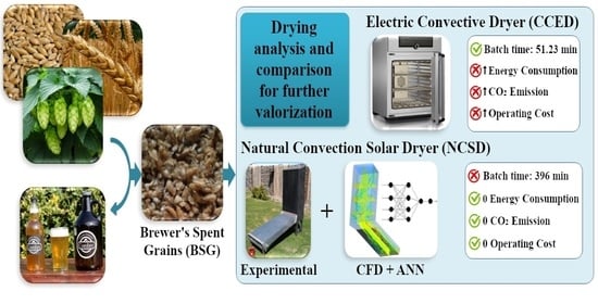
1. Introduction

The beer production market has been a highly concentrated one worldwide for a long time, with a substantial market share held by a few brewing companies which produce the most consumed industrial lager type of beer. Starting a decade ago, however, local microbreweries have been increasingly capturing the consumer’s interest with a wide range of different types of beer. The Argentinian beer industry does not escape this reality, and the craft beer market was growing 30% annually (pre-pandemic) [1]. Beer in all its variants is one of the most popular alcoholic beverages in the world. In Argentina in particular, its consumption began to grow steadily, reaching 2 · 10¹⁰ L/a [2].

Beer is made from sugars acquired from cereals and other grains (mainly barley and wheat), flavored and aromatized mostly with hops, but also with other herbs and additives, which are fermented in water with yeasts of the Saccharomyces type. In this process, large amounts of a solid fraction residue are produced, called brewer’s spent grains (BSG) [3], which form the most abundant byproduct of the brewing process, representing 85 % of the total residue and, on average, 31 % of the original weight of the malt spent in the process [4,5].

As a consequence of the appearance of microbreweries scattered around the country, large amounts of spent grains have been made available locally. The disposal of this residue is a serious environmental problem for communities and breweries because the volume of BSG generated is around 0.60 kg/L of beer brewed (as reported by the establishment which provided the samples and [6]). BSG are mainly used for animal feed; also, in a low fraction, for biogas generation; or are eliminated in landfills [7]. However, those byproducts potentially have several applications because of their year-round availability, low cost, and valuable chemical composition. The chemical composition is influenced by diverse factors like the grain used (barley, wheat, rice, corn, among others), processing method, harvesting time, and brewing conditions (i.e., the recipe used) [8]. Spent grains mainly consist of 15–26% protein and 70% fiber. The fiber consist of 16–25% cellulose, 28–35% hemicellulose, and 7–28% lignin [5].

Bolwig et al. [7] and Kavalopoulos et al. [9] studied the valorization of BSG as animal feed and biofuel, respectively, in the framework of biorefining and circular bioeconomy. Additionally, Fabani et al. [10] proposed a byproduct development process for watermelon rind in which rinds are transformed into nontraditional flour. Similarly, BSG are materials suitable for further valorization through such a process. For instance, BSG are added as an ingredient to enhance the fiber contents in recipes for pasta [11], bread, and snacks [3,12,13]. Recently, the potential use of BSG as fuel and food in Africa and its global warming capacity were studied by Maqhuzu et al. [14]. In addition, BSG can be used to directly recover fibers and antioxidant compounds [15].

Because of its high initial moisture (60–80%), transforming BSG from waste to raw materials requires a prior drying process. High moisture makes the product vulnerable to fast deterioration and spoilage within a few hours after brewing is over [16], and BSG at a disposal site like a landfill show an emission (expressed in CO₂ equivalents (CO_{2, eqv})) of 513 kg/t [9]. Currently, several devices are used for food dehydration, like hot air oven dryers and natural convection solar dryers (NCSD) [17,18]. The latter are economic to fabricate, reliable, environmentally friendly, and have lower operational costs than the former while being more efficient than direct sun dryers. In addition, solar drying reduces the CO_{2, eqv}, for instance, by reducing the use of conventional energy by as much as 80 % if forced convection is used [19]. Its working principle is based on sunrays directly heating the inlet air, thus lowering its humidity. Such an effect makes the air flow toward the dryer’s exhaust naturally. The passing air removes the moisture from the product on the trays and releases it into the outer atmosphere. An example can be found in [20] where a mixed-type solar dryer was successfully used for the dehydration of pear slices (Pyrus communis L.).

There is little information about BSG drying in the literature. Mallen and Najdanovic-Visak [21] studied the BSG drying kinetics at four temperatures (333.15 K, 343.15 K, 353.15 K, and 363.15 K) to extract biodiesel, while Kavalopoulos et al. [9] dehydrated BSG and milled them at the same time with a rotary drum food waste dryer at 378.15 K to produce biodiesel, bioethanol, and/or biogas.

The conventional modeling procedure for predicting the drying characteristic of a foodstuff is to use an existing empirical correlation based on a large number of experiments, like the Midilli model [10]. However, these correlations are frequently not sufficiently general to cover all particularities of the specific drying system [22]. One of the main problems that these models share is that their parameters have no physical meaning, and the only independent variable is the drying time. Consequently, there is no explicit relationship between the other operational variables (inputs) and the output. On the other hand, more complex models require the use of computational fluid dynamics (CFD). For instance, Sanghi et al. [23] developed a CFD model to simulate the corn drying process in an NCSD. Such a model successfully predicted the internal temperature, humidity, and air velocity profiles of the dryer. It was validated by using experimental information. Although the authors did not detail the simulation times needed to generate results, long computational times are a very important limitation because simulating even a few seconds of the drying process requires high computing power and time [24]. Instead, artificial neural networks (ANN) present an interesting alternative option. The training process of the ANN requires a relatively low number of datasets obtained from experiments, making it very efficient. The prediction of a new drying curve with a trained network is completed in seconds, thus avoiding time-consuming new experiments. Furthermore, expanding the neural model with new inputs and/or outputs is a very straightforward procedure. The most significant drawback of ANNs is that they can present poor results when attempting to perform extrapolations if limited data are available. Of course, these modeling approaches are not mutually exclusive and can be used together in order to achieve a synergetic effect between the local and global phenomena modeling and simulation.

One particular application of process models is the development of soft sensors, which are instruments capable of measuring difficult process variables indirectly [25], like moisture ratio (M_R). Ryniecki et al. [26] used a soft sensor based on a correlation for the determination of malting barley moisture ratio inside a fixed bed dryer. The purpose of the sensor was to allow the automation of the process through the prediction of the drying endpoint.

Objectives of This Work

This work aimed mainly to evaluate the NCSD as an alternative to electric convective dryers for the dehydration of local microbrewers’ spent grains. Two kinds of BSGGolden ale (GA) and Red ale (RA) were dried at different daytime hours in an NCSD. Furthermore, BSG were also dried in a conventional electric convectivedryer (CECD) at 333.15 K, 338.15 K, 343.15 K, 348.15 K, 353.15 K, 358.15 K, 363.15 K, and 368.15 K. Kinetic studies were completed for both drying methods. The measured dimensionless M_R values were modeled with eleven semitheoretical and empirical models for the CECD and, in turn, using CFD and ANNs for the NCSD. Finally, sustainability indices, specific energy consumption (e_C), and CO_{2, eqv} were calculated and used to consider the environmental impact of the NCSD with both its benefits and drawbacks.

2. Materials and Methods

2.1. Samples

The samples were provided by Cervecería Cumbre, San Juan Province, Argentina. They were collected after being removed from the maceration process of two types of beer: Golden ale (GA) and Red ale (RA) (Figure 1). Then, the samples were stored at 277.15 K in the dark until needed (no more than 1 or 2 days after sampling).

2.2. Analysis of the Samples

The moisture content, pH, and titratable acidity (citric acid content) were analyzed in the collected BSG (both raw and dried, i.e., initial and final values after drying) following the methodology of the AOAC (Official Methods of Analysis, 2010). All the analyses in fresh and dried BSG were repeated three times (N = 3) and the data gathered from them were expressed as the means ± standard deviation.

2.3. Drying Equipment and Experimental Procedure

In this subsection, first, both types of dryers are presented; second, the experimental procedures used with each one of them are described. In addition, the most important instrumentation equipment is described.

2.3.1. Conventional Electric Convective Dryer (CECD)

The convective BSG drying experiments were performed without pretreatment at eight different temperatures: 333.15 K, 338.15 K, 343.15 K, 348.15 K, 353.15 K, 358.15 K, 363.15 K, and 368.15 K, in an electric oven with a stainless-steel tube (0.12 m internal diameter and 1 m height), heated by the electrical resistance of 850 W. A complete description of this device was reported by Baldan et al. [27]. The air velocity was constant at 1 m/s during all the drying trials which were carried out until the average moisture content was lower than 10% according to the Codex Standard for wheat flour used for bakery and confectionery products (Codex Alimentarius, 1985 [28]) so as to prevent any degradation of the flour.

2.3.2. Natural Convection Solar Dryer (NCSD)

A solar dehydrator with natural airflow (Figure 2) was used for the BSG drying experiments which lasted until the moisture content was lower than 10% [28]. The product was placed on trays inside the solar dryer in layers of 0.5 cm thickness (Figure 2a). The drying experiments were carried out on two consecutive summertime days, each one in triplicate, with three full trays per trial. The weight of BSG used in each experiment was 0.265 kg per tray. Furthermore, each day, the experiments started at two different hours (8:30 and 11:00 in the morning) to analyze the influence of irradiance and ambient temperature on the drying process of the samples. The morning time was selected considering that at 8:30 a.m. the irradiance value is minimal while at 11:00 a.m. a steady increase in irradiance (slope) begins and is sustained over time. Weight loss data was registered at different time intervals during the drying process until a constant weight was obtained. The measurements were performed by taking the trays from the chamber in regular intervals to be weighted with a balance Compass CR621 (OHAUS, Parsippany, United States). The drying chamber was 1.32 m in height, 0.56 m in width, and 0.33 m in depth. The collector was 1.24 m in length, 0.56 m in width, and 0.15 m in depth (Figure 2b). The cover of the collector (upper part) was transparent and made of a material that allowed the passage of solar energy, minimal loss of sunlight waves, and was resistant to inclement weather. In this case, 150 µm polyethylene was used. The drying system was classified as a natural convection indirect type, and the angle of inclination of the collector was set to 10° (Figure 2C). Although the Sun’s position could have allowed an optimum inclination of between 30° and 50° [29], a very conservative value of 10° was selected to not overheat BSG according to the values of irradiance obtained in San Juan Province where the experiments were performed. The maximum and minimum temperatures achievable by the solar dryer were, approximately, between 318.55 K and 291.85 K, respectively.

The final moisture content of samples was determined using a PMR50 analyzer (Radwag, Radom, Poland) at 378.15 K [30]. The dried samples were stored at a temperature of around 293.15 K in a dark room until needed for analysis within 14 d after drying. All the analyses were performed in triplicates, and the data gathered from them were expressed as the means ± standard deviation. The irradiance values were measured with a solar power meter model TM-206 (TENMARS, Taipei, Taiwan).

2.4. Mathematical Modeling of Drying Curves

M_R was calculated with the experimental results obtained from the drying trials [31]. The drying curves of BSG (M_R(t)) were modeled using 11 different empirical models taken from the literature [32]. To assess the goodness of fit of the applied models with the experimental data, the statistical indicators chi-squared (χ²), sum of squared errors (S_SE), and root-mean-square error (µ_RSE) were used. The models with lower values of χ², S_SE, and µ_RSE have a better fitting performance, while a value of R² closer to unity is more desirable.

2.5. Specific Energy Consumption and CO₂ Emissions

The high energy consumption of dryers also influences greenhouse gas emissions and has environmental consequences, which is very important [33]. Nowadays, scientists are looking for solutions that reduce energy consumption and CO₂ emissions using different pretreatment methods or adjusting the methods and parameters of drying to obtain the best results [34]. For that, e_C and CO_{2, eqv} were used to compare the CECD and the NCSD. Firstly, for e_C, with Equation (1), the energy needed to dry 1 kg of fresh BSG was calculated [35]. Secondly, since in Argentina the electric energy supply for the CECD is provided by a mixture of nonrenewable and renewable sources (natural gas, thermal power, hydropower, and wind, among others) the electricity CO_{2, eqv} is 0.358 3 kg/(kW h) according to Climate Transparency 2019 [36]. Thus, to calculate the CO_{2, eqv} $(\mathrm{expressed} \mathrm{in} \mathrm{kg}/(\mathrm{kW} \mathrm{h}\left)\right)$ needed to dry 1 kg of BSG, the calculated e_C values have to be multiplied by this constant (Equation (2)).

$$e_{\mathrm{C}}{=(c}_{p,\mathrm{a}}{+c}_{p,\mathrm{v}}{\mathrm{h}}_{\mathrm{a}})\frac{{qt(T}_{\mathrm{in}}-T_{\mathrm{am}})}{m_{\mathrm{v}}{V}_{\mathrm{h}}}$$

(1)

$${\mathrm{CO}}_{2, \mathrm{eqv} }=0.358 3 · e_{\mathrm{C}}$$

(2)

2.6. Modeling and Simulation of the Solar Drying Process

The main reason for developing computational models of the solar drying process is to be able to predict the behavior of M_R evolution based on the main independent variables of the process like irradiance, initial moisture content (w_IM), and others under different conditions without the need for so much experimental work. Needless to say, the conventional electric drying process is less subject to upsets in independent variables because it is carried out in an indoor controlled environment/system, whereas the solar drying process is carried out in an outdoor environment, without control of the main independent variables. The conventional electric drying process modeling is covered in Section 2.4.

2.6.1. CFD–ANN Complementary Modeling Approach

Two complementary techniques were applied to model and simulate the behavior of the solar dryer under different conditions: computational fluid dynamics (CFD) and artificial neural networks (ANN). This is because neither of them can singlehandedly model and simulate both the local and global phenomena of solar dryers efficiently. CFD can accurately and efficiently predict the temperature gradient, air velocity, and other variables inside the solar dryer, whereas it is very costly computationally to model and simulate the global drying phenomenon (i.e., M_R evolution). The latter is easily modeled and simulated by an ANN based on a handful of experimental data, whereas the former would need plenty of experiments to generate sufficient data to train a good ANN model.

Further complementation could also be achieved because the CFD model can generate the irradiance values of each day of the year for any particular latitude and longitude. These data could be applied as training data and simulation input for the ANN model without the need for hourly and daily actual measurements. This kind of complementation would be useful in a future expansion of the ANN model to cover daily and seasonal changes in solar drying curves. Such a project would need more drying experiments distributed around the year.

2.6.2. CFD Modeling

The analysis was performed by solving basic fluid governing equations (continuity, momentum, and energy) by using the finite volume method (FVM). The simulations were carried out with ANSYS Fluent® 18.1 (ANSYS, Canonsburg, PA, USA) using a ray-tracing analysis. With this technique, we simulated the interaction between solar rays and the solar collector to quantify the amount of energy that impinges on the receiver at a particular daytime. The governing equations are summarized, for instance, in the work of Sanghi et al. [23]. The solar dryer’s geometrical setup and boundary conditions adopted are shown in Figure 3.

A polyhedral mesh was applied with 77,090 cells. Mesh validation with experimental results showed that no significant improvement was obtained by adding more cells to the mesh. A k-epsilon turbulence model was used. All the simulations were performed in the steady state and the reverse flow in the outlet was disabled.

2.6.3. ANN Modeling

Since San Juan Province has a very dry climate with low humidity, the main drivers of the drying process are the irradiance values and w_IM of the lot. A solar drying chamber does not have a fairly constant controlled internal temperature as a conventional electric convective dryer. Instead, it presents a temperature gradient that is subject to the Sun’s irradiance variations (as shown in the CFD simulations). These particularities set the ANN’s input/output design as shown in Figure 4.

Once the number of inputs and outputs is established based on the experimental data available, the design of the ANN model involves the selection of the network type, the activation functions, the number of hidden layers, and the number of neurons in each one. Regarding the choice of network and neuron types, the universal approximation theorem (Pinkus [37]) establishes that multilayer perceptron networks with at least one hidden layer and a nonlinear activation function are universal approximators that can fit any given polynomial. In addition, for some models, deeper networks can work better than single-hidden-layer networks (no more than two hidden layers, most likely).

The process of selecting the number of hidden layers and the number of neurons in each one was carried out by trial-and-error. First, single-hidden-layer networks with as few as three neurons showed good performance (R² > 0.999). Increasing the number of hidden neurons to amounts of more than seven proved to show signs of overfitting when prediction tests of drying curves were performed. These prediction tests involved drying curves with different values of w_IM, batch starting hour, and batch times. Particularly, adding a second hidden layer helped in fitting the batch times better. The final model selection was performed according to the algorithm presented by Fabani et al. [10]. The complete set of ANN parameters is shown in

Table 1. Complete set of Artificial neural networks (ANN) parameters.

Parameter	Value
Network type	Multilayer feedforward (MLFF)
Neuron type	Perceptron
Inputs	4
Output	1 (moisture ratio)
Normalization type	Min–Max
Activation function	Sigmoid (hidden) and linear (output)
Training algorithm	Bayesian regularization backpropagation *
Training sets	264
Number of hidden layers	2
Number of neurons per layer	4 and 1
Train ratio	97%
Validation ratio	N/A **
Test ratio	3%

* This particular training algorithm’s stop condition is the maximum number of epochs. ** N/A: not applicable.

. Finally, the MATLAB^® (MathWorks®, Natick, MA, USA) release 2016a, Neural Fitting Tool was used to design, train weights and biases, test and implement the ANN model.

2.6.4. ANN Simulations

One of the main independent variables which directly affect the batch time is the average w_IM of the sample. Additionally, the starting daytime hour (SDTH) of the drying process directly affects the drying rate (v_D) because the amount of power the Sun provides is not constant. These two factors can shorten or extend the drying batch duration so it is paramount to determine how they can affect the total yield. The consequences of variations in these two variables were determined using ANN simulations which, in turn, were used to calculate the indicators in Equations (3) and (4): the average first batch time duration (t_B1) and the average second batch duration (t_B2), both for any given starting daytime hour.

$${\overline{t_{\mathrm{B}1}}}_{\mathrm{SDTH}}{=10}^{-1} ·{\displaystyle \sum }_{w_{\mathit{I}\mathit{M}}=64}^{74}{t}_{\mathrm{B}1}{}_{w_{\mathit{I}\mathit{M}}}$$

(3)

$${\overline{t_{\mathrm{B}1}}}_{\mathrm{SDTH}}{=10}^{-1} ·{\displaystyle \sum }_{w_{\mathit{I}\mathit{M}}=64}^{74}{t}_{\mathrm{B}1}{}_{w_{\mathit{I}\mathit{M}}}$$

(4)

The simulations were performed considering that the first batch can start as early as 08:30 in the morning and that the second batch starts a half-hour after the first one finishes. The batch stop condition is M_R lower than 0.1. Finally, due to the experimental results, only two full batches are expected. It is important to mention that since the ANN model is data-based, the validity of its results is limited to the day the drying experiments were carried out. On the other hand, the CFD model can produce simulation results of any day of the year.

2.7. Statistical Performance Indicators

Firstly, the goodness of fit between the empirical models and the experimental data was assessed based on the chi-squared (χ²) statistical indicator, the sum of squared errors (S_SE), and the mean squared error (µ_SE):

$${\chi }^2={\displaystyle \sum }_{i=1}^{\mathrm{N}}\frac{{(M}_{\mathrm{R} }{}_{\mathrm{pre},i}-M_{\mathrm{R} }{}_{\exp ,i}{) }^2}{M_{\mathrm{R} }{}_{\exp ,i}}$$

(5)

$$S_{\mathrm{SE}}={\displaystyle \sum }_{i=1}^{\mathrm{N}}{{(M}_{\mathrm{R} }{}_{\mathrm{pre},i}-M_{\mathrm{R} }{}_{\exp ,i})}^2$$

(6)

$${\mu }_{\mathrm{SE}}=\frac{1}{\mathrm{N}} · {\displaystyle \sum }_{i=1}^{\mathrm{N}}{{(M}_{\mathrm{R} }{}_{\mathrm{pre},i}-{ M}_{\mathrm{R} }{}_{\exp ,i})}^2$$

(7)

Secondly, the evaluation of the ANNs performance was based on two statistical indicators: µ_SE (Equation (7)) and the coefficient of determination R²:

$$R^{2 }=1 -\left[\frac{{{\displaystyle \sum }}_{i=1}^{\mathrm{N}}{\left(M_{\mathrm{R} }{}_{\mathrm{pre},\mathrm{i}}-M_{\mathrm{R} }{}_{\exp ,i}\right)}^2}{{{\displaystyle \sum }}_{i=1}^{\mathrm{N}}{\left({\overline{M_{\mathrm{R} }}}_{\mathrm{pre},i}-M_{\mathrm{R} }{}_{\exp ,i}\right)}^2}\right]$$

(8)

Unlike χ² and µ_SE, R² values closer to unity are more desirable, show better fitting performance. Additionally, the R² indicator is more commonly associated with the software applications used to train ANNs.

Finally, in this work, units and quantities were mentioned according to the International System of units (SI) and compatible units as reported by Glavič [38].

3. Results

3.1. Raw and Dried Moisture, pH and Titratable Acidity of the Samples

The fresh samples of BSG presented high w_IM values, which were 64.3 ± 0.2% for BSG-GA and 74.2 ± 0.5% for BSG-RA, all within the previously reported range of 60–90% mass [18]. Secondly, the fresh samples presented pH values of 5.63 ± 0.08 for the GA variety and 6.06 ± 0.05 for the RA variety, while the titratable acidity values (expressed in % citric acid) were 0.40 ± 0.02% and 0.37 ± 0.02%, respectively.

The samples dried in the CECD presented the final moisture content values of less than 7 % and final pH and acidity values which varied according to the temperature value used, ranging from 5.4 to 5.8 and from 0.65% to 1.10%, respectively. On the other hand, the final moisture content of the sun-dried BSG was less than 6–7%, pH was 5.49 ± 0.06 for the GA variety and 5.62 ± 0.02 for the RA variety, and, finally, the titratable acidity values (expressed in % citric acid) were 0.56 ± 0.05% and 0.52 ± 0.01% for GA and RA, respectively.

In

Table 2. Summary of the analytical results.

	Fresh Samples			Dried Samples: CECD			Dried Samples: NCSD
Variety	wM (%)	pH	Titratable Acidity (% Citric Acid)	wM (%)	pH	Titratable Acidity (% Citric Acid)	wM (%)	pH	Titratable Acidity (% Citric Acid)
Golden ale	64.3 ± 0.2	5.63 ± 0.08	0.40 ± 0.02	6.52 ± 0.16	5.42 ± 0.08	0.86 ± 0.18	6.42 ± 0.21	5.49 ± 0.06	0.56 ± 0.05
Red ale	74.2 ± 0.5	6.06 ± 0.05	0.37 ± 0.02	6.78 ± 0.13	5.71 ± 0.24	0.55 ± 0.05	6.30 ± 0.27	5.62 ± 0.02	0.52 ± 0.01

, a summary of the analytical results is shown. Both driers presented similar values for moisture content and pH of the dried samples, while the NCSD presented improved values of titratable acidity compared to the CECD. The titratable acidity values of the samples dried in the NCSD were lower, closer to those of the fresh samples. This particular indicator is important because it is related to the flavor of a foodstuff. The NCSD samples had lower values (improved organoleptic quality indices) than the CECD ones at all the temperatures assessed. Dzelagha et al. [39] obtained similar results when studying different drying technologies and the effect on bean quality parameters. These could be related to the significant increment of free fatty acid and acetic acid levels with the rising temperature which, in turn, was proportional to the corresponding decrease in pH, suggesting the optimal oven temperature of 318.15 K. Moreover, certain vitamins are broken down at high temperatures, such as vitamin C, thus diminishing their content [32].

3.2. Drying Characteristics of BSG

The drying curves of BSG, GA and RA varieties, in the CECD and the NCSD were modeled with empirical and ANN models, respectively. The CECD experimental drying curves showed an exponential decay with the first phase where the moisture is rapidly lost (high drying rates) and the second phase that presented low drying rates until the samples reached low moisture contents (Figure 5a). In addition, the drying rates increased with temperature due to the increased heat transfer between the circulating air and the BSG, favoring water evaporation. The drying models which fitted the experimental data best were, first, the Midilli model (S_SE = 4.1 · 10⁻⁵; µ_RSE = 6.2 · 10⁻³, and χ² = 4.3 · 10⁻⁵), and, second, the two-term model (S_SE = 6.6 · 10⁻⁵; µ_RSE = 7.9 · 10⁻³, and χ² = 6.9 · 10⁻⁵). Therefore, based on the statistical indicators presented, the Midilli model is more accurate to predict the M_R evolution for the CECD.

The NCSD showed greater efficiency when the drying process was started at 11:00 in the morning, achieving a decrease in moisture content in a shorter time interval for the two varieties studied (Figure 5b). The experiments that started at 11:00 achieved a reduced drying time (M_R lower than 0.1) from 420 min to 345 min for the GA variety and from 430 min to 390 min for the RA variety when compared with those that started at 08:00. The ANN model’s fitting performance had R² > 0.999 and µ_RSE = 4.25 · 10⁻³. In the solar bagasse drying, a greater variation in the drying rate (more peaks) was observed compared to the convection bagasse drying.

3.3. Comparative Analysis of the CECD and the NCSD

In

Table 3. Results of the conventional convective drying process of the raw matter: Golden ale.

Drying Temperature (K)	Batch Time (min)	wM (%)	Total Energy Consumption (kW h)	Removed Water (g)	eC ((kW h)/kg)	CO2, eqv (kg/(kW h))	Electricity Cost (USD/kg)
333.15 ± 0.20	84.33 ± 5.48	6.79 ± 0.21	0.29 ± 0.02	1.68 ± 0.03	407.58 ± 26.76	158.14 ± 10.38	1.02 ± 0.07
338.15 ± 0.20	64.50 ± 1.32	6.70 ± 0.11	0.24 ± 0.01	1.60 ± 0.03	376.13 ± 15.34	145.94 ± 5.95	0.94 ± 0.04
343.15 ± 0.20	54.33 ± 1.26	6.60 ± 0.09	0.22 ± 0.01	1.61 ± 0.06	352.48 ± 7.46	136.76 ± 2.89	0.88 ± 0.02
348.15 ± 0.20	50.81 ± 3.01	6.52 ± 0.12	0.22 ± 0.01	1.66 ± 0.02	356.47 ± 16.33	138.31 ± 6.33	0.89 ± 0.04
353.15 ± 0.20	46.17 ± 3.55	6.45 ± 0.08	0.21 ± 0.02	1.73 ± 0.08	341.80 ± 10.81	132.62 ± 4.19	0.85 ± 0.03
358.15 ± 0.20	40.17 ± 2.08	6.40 ± 0.05	0.19 ± 0.01	1.64 ± 0.04	341.72 ± 12.27	132.59 ± 4.76	0.85 ± 0.03
363.15 ± 0.20	35.5 ± 1.04	6.38 ± 0.12	0.18 ± 0.01	1.68 ± 0.01	320.86 ± 7.13	124.49 ± 2.77	0.80 ± 0.05
368.15 ± 0.20	34.17 ± 2.02	6.34 ± 0.09	0.18 ± 0.01	1.88 ± 0.06	296.44 ± 18.89	115.02 ± 7.33	0.74 ± 0.05

and

Table 4. Results of the conventional convective drying process of the raw matter: Red ale.

Drying Temperature (K)	Batch Time (min)	wM (%)	Total Energy Consumption (kW h)	Removed Water (g)	eC ((kW h)/kg)	CO2, eqv (kg/(kW h))	Electricity Cost (USD/kg)
333.15 ± 0.20	71.50 ± 3.91	6.94 ± 0.14	0.24 ± 0.01	1.49 ± 0.09	391.95 ± 39.39	152.08 ± 15.28	0.98 ± 0.10
338.15 ± 0.20	69.83 ± 4.25	6.91 ± 0.16	0.26 ± 0.02	1.80 ± 0.01	360.22 ± 23.97	139.76 ± 9.30	0.90 ± 0.06
343.15 ± 0.20	59.50 ± 0.90	6.87 ± 0.13	0.24 ± 0.01	1.89 ± 0.03	331.83 ± 5.12	128.75 ± 1.99	0.83 ± 0.01
348.15 ± 0.20	58.17 ± 0.58	6.82 ± 0.14	0.25 ± 0.01	1.94 ± 0.08	350.23 ± 17.69	135.89 ± 6.86	0.88 ± 0.04
353.15 ± 0.20	45.17 ± 1.89	6.77 ± 0.20	0.20 ± 0.01	1.65 ± 0.20	353.12 ± 29.74	137.01 ± 11.54	0.88 ± 0.07
358.15 ± 0.20	43.00 ± 0.50	6.71 ± 0.12	0.21 ± 0.01	1.69 ± 0.04	354.41 ± 10.63	137.51 ± 4.12	0.89 ± 0.03
363.15 ± 0.20	36.00 ± 3.28	6.67 ± 0.09	0.18 ± 0.02	1.64 ± 0.01	330.27 ± 27.89	128.14 ± 10.82	0.83 ± 0.07
368.15 ± 0.20	33.17 ± 2.75	6.54 ± 0.10	0.17 ± 0.01	1.57 ± 0.03	328.80 ± 17.77	127.57 ± 6.89	0.82 ± 0.04

, the results of the CECD process of the raw product are presented. Both varieties of the BSG were dried at eight different temperatures, from 333.15 K to 368.15 K. As expected, from the environmental impact indicators’ point of view, there were no significant differences. Both ales presented similar values for e_C and CO_{2, eqv}, averaging 346.92 (kW h)/kg and 124.30 kg/(kW h) for e_C and CO_{2, eqv}, respectively. Similar values of the operational indicators are also shown for both varieties, averaging 51.23 min of batch time and 0.86 USD of electricity per kilogram of raw product. In conclusion, from that single perspective only, higher drying temperatures are more efficient.

In

Table 5. Results of the solar drying process of the raw matter for Golden ale and Red ale.

BSG	Daytime Hour	Batch Time (min)	eC ((kW h)/kg)	CO2, eqv (kg/(kW h))	Electricity Cost (USD/kg)
Golden ale	08:30	420	0.00	0.00	0.00
Golden ale	11:00	345	0.00	0.00	0.00
Red ale	08:30	430	0.00	0.00	0.00
Red ale	11:00	390	0.00	0.00	0.00

, the solar dryer’s results of the drying process of the raw product are shown. The experiments were conducted during the austral summer at two different daytime hours, 08:00 and 11:00, for each type of the BSG. The results showed an average batch time of 396 min, with the RA type exhibiting slightly longer drying times due to its higher w_IM compared to the GA variety. Additionally, the NCSD has null operating costs because solar energy is freely available and there is no forced airflow. Consequently, both environmental impact indicators have null values, too. In

Table 6. Summary of indicators.

	Conventional Electric Convective Dryer (CECD)	Natural Convection Solar Dryer (NCSD)
Average drying temperature (K)	350.65	319.65
Average batch time (min)	51.23	396.00
Average eC ((kW h)/kg)	346.92	0.00
Average CO2, eqv (kg/(kW h))	124.30	0.00
Average operating cost (USD/kg)	0.86	0.00

, a summary of the most important environmental and process indicators previously explained is presented.

3.4. CFD Simulation Results

Aiming to validate the CFD computational model, temperature measurements were performed inside the empty drying chamber under different irradiance conditions during the springtime, before the experiments.

Table 7. CFD simulations’ results and experimental validations.

					Temperature (K)
Daytime Hour	Ambient Temperature (K)		Solar Irradiance (W/m2)		Point 1		Point 2		Point 3
	EXP	CFD	EXP	CFD	EXP	CFD	EXP	CFD	EXP	CFD
12:30	299.65	299.15	1005	944.63	305.75	309.28	307.95	309.07	309.65	308.87
14:00	302.75	299.15	1040	945.46	312.65	312.48	313.15	312.15	314.45	311.84
15:30	303.75	299.15	860	928.91	312.75	316.12	312.85	315.82	312.85	315.54

shows the temperature measurements performed in the lower section of the chamber (point 1), in the middle section of the chamber (point 2), and the upper section of the chamber near the exit (point 3) at three different daytime hours. Additionally, the corresponding simulation results are shown, indicating a good agreement between the simulated values and the measured ones (Table 7). The minimal differences can be attributed to deviations in the model’s irradiance values, and it is also important to consider that the lower wall of the dryer exchanges heat with the surrounding environment (heat transfer coefficient adopted for simulations = 10 W/(m² K)), rendering the temperature in the drying chamber lower than the temperature in the solar heating section.

Once the CFD model was validated, simulations were performed to assess how both seasonal changes and daytime hour changes affect the temperature gradient inside the drying chamber. In Figure 6, four longitudinal cutaways of the drying chamber are presented, also under four different irradiance conditions. The calculated mean temperatures were as follows: 309.55 K for a summer morning (11:00); 312.58 K for a summer afternoon (15:00); 306.81 K for a winter morning (11:00); and 309.23 K for a winter afternoon (15:00).

3.5. ANN Simulation Results 1: The Effect of Irradiance and w_IM in the Drying Rates

The drying rate of the sample inside the drying chamber is controlled by the rate at which heat is applied to it (i.e., power applied), the rate at which the sample’s internal moisture is released from its surface, and the rate at which moist air is removed from the drying chamber. Regarding the power applied, in a conventional electric dryer, once the chamber’s internal temperature is constant, the power consumption is constant, too, whereas in the solar dryer, the available power per square meter (irradiance) varies throughout the day and is only controlled by the Earth’s rotation. Therefore, the drying rates during the several known stages of the process vary if the same sample starts drying early in the morning or early in the afternoon, for instance.

It can be seen from the experimental curves (Figure 5b) that the slope of those samples that started drying at 08:30 was less steep than the slope of those that started drying at 11:00 during the constant drying rate stage. Additionally, the ANN predictions in Figure 7 show that the samples which start drying later in the afternoon show an even steeper slope during the constant drying rate stage as the irradiance values continue to rise. This is because the bulk of the water is easier to remove and because the irradiance values are very high. Then, the drying rate slows down because both the remaining water is harder to remove and the irradiance values rapidly start to fall. In comparison, the drying rate of the samples which started at 08:30 is pretty constant throughout because when the irradiance values start to climb, the remaining water is harder to remove, and vice versa.

Finally, the ANN predictions also show the effect of w_IM of the samples. In Figure 7, it can be seen that a sample with a w_IM of 70% (a value which is in between the GA and the RA) had a batch time that was shorter than the RA but longer than the GA for both the curves which started early in the morning and later in the afternoon. Other curves with w_IM values within that same range showed a similar behavior.

3.6. ANN Simulation Results 2: Average Batch Durations

As the experimental results suggest, only two full batches can be completed per day with the measured irradiance values and w_IM. Therefore, simulations were performed to determine how w_IM and the starting daytime hour affect batch times. This is another indicator of how the irradiance controls the drying process and its potential total yield.

Applying all the simulation results to Equations (3) and (4), the plots of Figure 8 were obtained. The results show that both average batch duration curves—which depend on the starting daytime hour—have the opposite slope of the irradiance curve, meaning that as long as the irradiance rises, the batch durations fall, and vice versa. The total batch time curve (batch 1 plus batch 2) also presents a similar shape. The results also show that the first batch can start as late as 11:30 in the morning to complete two full batches in the same day. Finally, simulations were used to calculate the mean batch time for every w_IM in the 64–74% range and for every SDTH. The result was a mean batch time of 366 min as shown in Table 4, 30 min slower than the obtained experimental value. This difference could be because many more curves were used from the simulation to calculate these indicators.

4. Discussion and Conclusions

A natural convection solar dryer (NCSD) was evaluated as an alternative to a conventional electric convective drying system (CECD) for the dehydration process of local microbrewers’ spent grains. For the different drying temperatures (333.15–363.15 K), e_C and CO_{2, eqv} for the CECD varied between 1.68 · 10⁻³ (kW h)/kg and 1.88 · 10⁻³ (kW h)/kg and between 294.80 kg/(kW h) and 410.73 kg/(kW h); however, using the NCSD, both indicators were null. From the environmental management perspective, the NCSD does not need any grid energy to function and eliminates 100% of the CO_{2, eqv}. Thus, if labor costs are not considered, the overall operating costs are greatly reduced. Secondly, the NCSD produces a dried product with a comparatively better quality, as shown by the lower titratable acidity values. Lastly, another important aspect is the cost of the equipment itself (initial investment). The NCSD is about 40–45% cheaper than the CECD.

On the other hand, the most important disadvantage of the NCSD is the fact that batch times (345–430 min, depending on the starting daytime hour at which the drying process begins) are much longer, consequently reducing the total yield. In light of this, it is of paramount importance to find tools that help operators find the optimal conditions in which to work to make the NCSD more appealing. Through simulations, the importance of the Sun’s irradiance was measured under conditions different from those of the experiments. It was established with the ANN model how the irradiance values directly govern the drying rates and the average batch times. Moreover, the developed CFD model can produce irradiance values via simulations for any location on the planet where the same solar dryer could be placed regardless of the day and time of the year. The internal temperature gradients were obtained under several conditions. This information can be used to determine the optimal operating conditions for the solar dryer to get the highest possible yield of dried BSG. These results further show the contrast between both drying methods. In an electric convective dryer, the operating variables adapt themselves to the operator’s needs and, on the other hand, in the NCSD, the operator has to adapt to the operating conditions. Consequently, these simulation tools can further assist the solar drying process by using them to develop soft sensors, which are instruments that can, for instance, determine the drying endpoint.

Future work should include, as the first step, the optimization of the drying process based on the technofunctional properties of the flour obtained by milling dried BSG using the response surface methodology.

References

- Díaz, M.; Cabello, X. (Eds.) South American Brewery Yearbook, 1st ed.; Ediciones Inter Andina: San Carlos de Bariloche, Argentina, 2016. [Google Scholar]
- FAO. Production Quantities of Beer by Country. Food and Agriculture Organization of the United Nations. FAOSTAT, Food and Agriculture Data. 2021. Available online: https://www.fao.org/faostat/en/#data/FBS (accessed on 12 December 2021).
- Lynch, K.M.; Steffen, E.J.; Arendt, E.K. Brewers’ spent grain: A review with an emphasis on food and health. J. Inst. Brew. 2016, 122, 553–568. [Google Scholar] [CrossRef]
- Nigam, P.S. An overview: Recycling of solid barley waste generated as a by-product in distillery and brewery. Waste Manag. 2017, 62, 255–261. [Google Scholar] [CrossRef] [PubMed]
- Steiner, J.; Procopio, S.; Becker, T. Brewer’s spent grain: Source of value-added polysaccharides for the food industry in reference to the health claims. Eur. Food Res. Technol. 2015, 241, 303–315. [Google Scholar] [CrossRef]
- Ministry of Agriculture, Argentine Republic. Available online: http://www.alimentosargentinos.gob.ar/HomeAlimentos/Nutricion/documentos/TendenciaBagazo.pdf (accessed on 10 December 2021).
- Bolwig, S.; Mark, M.S.; Happel, M.K.; Brekke, A. Beyond animal feed?: The valorisation of brewers’ spent grain. In From Waste to Value. Valorisation Pathways for Organic Waste Streams in Circular Bioeconomies, 1st ed.; Taylor & Francis: Abingdon, UK, 2019; pp. 107–126. [Google Scholar] [CrossRef]
- Mussatto, S.I. Brewer’s spent grain: A valuable feedstock for industrial applications. J. Sci. Food Agric. 2014, 94, 1264–1275. [Google Scholar] [CrossRef] [PubMed] [Green Version]
- Kavalopoulos, M.; Stoumpou, V.; Christofi, A.; Mai, S.; Barampouti, E.M.; Moustakas, K. Sustainable valorisation pathways mitigating environmental pollution from brewers’ spent grains. Environ. Pollut. 2021, 270, 116069. [Google Scholar] [CrossRef] [PubMed]
- Fabani, M.P.; Capossio, J.P.; Román, M.C.; Zhu, W.; Rodriguez, R.; Mazza, G. Producing non-traditional flour from watermelon rind pomace: Artificial neural network (ANN) modeling of the drying process. J. Environ. Manag. 2021, 281, 111915. [Google Scholar] [CrossRef] [PubMed]
- Nocente, F.; Taddei, F.; Galassi, E.; Gazza, L. Upcycling of brewers’ spent grain by production of dry pasta with higher nutritional potential. LWT 2019, 114, 108421. [Google Scholar] [CrossRef]
- Aliyu, S.; Bala, M. Brewer’s spent grain: A review of its potentials and applications. Afr. J. Biotechnol. 2011, 10, 324–331. [Google Scholar] [CrossRef]
- Ktenioudaki, A.; Crofton, E.; Scannell, A.G.M.; Hannon, J.A.; Kilcawley, K.N.; Gallagher, E. Sensory properties and aromatic composition of baked snacks containing brewer’s spent grain. J. Cereal Sci. 2013, 57, 384–390. [Google Scholar] [CrossRef]
- Maqhuzu, A.B.; Yoshikawa, K.; Takahashi, F. Prospective utilization of brewers’ spent grains (BSG) for energy and food in Africa and its global warming potential. Sustain. Prod. Consum. 2021, 26, 146–159. [Google Scholar] [CrossRef]
- Vadivel, V.; Moncalvo, A.; Dordoni, R.; Spigno, G. Effects of an acid/alkaline treatment on the release of antioxidants and cellulose from different agro-food wastes. Waste Manag. 2017, 64, 305–314. [Google Scholar] [CrossRef]
- Fărcaş, A.C.; Socaci, S.A.; Mudura, E.; Dulf, F.V.; Vodnar, D.C.; Tofană, M. Exploitation of Brewing Industry Wastes to Produce Functional Ingredients. Brew Technol. 2017, 1, 137–156. [Google Scholar] [CrossRef] [Green Version]
- Fabani, M.P.; Román, M.C.; Rodriguez, R.; Mazza, G. Minimization of the adverse environmental effects of discarded onions by avoiding disposal through dehydration and food-use. J. Environ. Manag. 2020, 271, 110947. [Google Scholar] [CrossRef] [PubMed]
- Chavan, A.; Vitankar, V.; Mujumdar, A.; Thorat, B. Natural convection and direct type (NCDT) solar dryers: A review. Dry. Technol. 2021, 39, 1969–1990. [Google Scholar] [CrossRef]
- Udomkun, P.; Romuli, S.; Schock, S.; Mahayothee, B.; Sartas, M.; Wossen, T. Review of solar dryers for agricultural products in Asia and Africa: An innovation landscape approach. J. Environ. Manag. 2020, 268, 110730. [Google Scholar] [CrossRef]
- Lopez-Vidaña, E.C.; Cesar-Munguía, A.L.; García-Valladares, O.; Salgado Sandoval, O.; Dominguez Niño, A. Energy and exergy analyses of a mixed-mode solar dryer of pear slices (Pyrus communis L.). Energy 2021, 220, 119740. [Google Scholar] [CrossRef]
- Mallen, E.; Najdanovic-Visak, V. Brewers’ spent grains: Drying kinetics and biodiesel production. Bioresour. Technol. Rep. 2018, 1, 16–23. [Google Scholar] [CrossRef] [Green Version]
- Topuz, A. Predicting moisture content of agricultural products using artificial neural networks. Adv. Eng. Softw. 2010, 41, 464–470. [Google Scholar] [CrossRef]
- Sanghi, A.; Ambrose, R.P.K.; Maier, D. CFD simulation of corn drying in a natural convection solar dryer. Dry. Technol. 2018, 36, 859–870. [Google Scholar] [CrossRef]
- Malekjani, N.; Jafari, S.M. Simulation of food drying processes by Computational Fluid Dynamics (CFD); recent advances and approaches. Trends Food. Sci. Technol. 2018, 78, 206–223. [Google Scholar] [CrossRef]
- Kadlec, P.; Gabrys, B.; Strandt, S. Data-driven Soft Sensors in the process industry. Comput. Chem. Eng. 2009, 33, 795–814. [Google Scholar] [CrossRef] [Green Version]
- Ryniecki, A.; Gawrysiak-Witulska, M.; Wawrzyniak, J. Correlation for the automatic identification of drying endpoint in near-ambient dryers: Application to malting barley. Biosyst. Eng. 2007, 98, 437–445. [Google Scholar] [CrossRef]
- Baldán, Y.; Fernandez, A.; Reyes Urrutia, A.; Fabani, M.P.; Rodriguez, R.; Mazza, G. Non-isothermal drying of bio-wastes: Kinetic analysis and determination of effective moisture diffusivity. J. Environ. Manag. 2020, 262, 110348. [Google Scholar] [CrossRef] [PubMed]
- Codex Alimentarius. Codex Standard for Wheat Flour. CXS 152-1985.: International Food Standards. Revised in 1995. Amended in 2016. 2019. Available online: http://www.fao.org/fao-who675codexalimentarius (accessed on 13 December 2021).
- Zhang, H.L.; Baeyens, J.; Degreve, J.; Caceres, G. Concentrated solar power plants: Review and design methodology. Renew. Sust. Energ Rev. 2018, 22, 466–481. [Google Scholar] [CrossRef]
- AOAC. Official Methods of Analysis of AOAC International, 18th ed.; AOAC International: Gaithersburg, MD, USA, 2010; ISBN 0-935584-80-3. Available online: http://www.eoma.aoac.org/ (accessed on 3 November 2021).
- Praveen Kumar, D.G.; Hebbar, H.U.; Ramesh, M.N. Suitability of thin layer models for infrared-hot air-drying of onion slices. LWT Food Sci. Technol. 2006, 39, 700–705. [Google Scholar] [CrossRef]
- Roman, M.C.; Fabani, M.P.; Luna, L.C.; Feresin, G.E.; Mazza, G.; Rodriguez, R. Convective drying of yellow discarded onion (Angaco INTA): Modelling of moisture loss kinetics and effect on phenolic compounds. Inf. Process Agric. 2020, 7, 333–341. [Google Scholar] [CrossRef]
- Nabavi-Pelesaraei, A.; Rafiee, S.; Mohtasebi, S.S.; Hosseinzadeh-Bandbafha, H.; Chau, K. Integration of artificial intelligence methods and life cycle assessment to predict energy output and environmental impacts of paddy production. Sci. Total Environ. 2018, 631–632, 1279–1294. [Google Scholar] [CrossRef] [PubMed]
- Witrowa-Rajchert, D.; Wiktor, A.; Sledz, M.; Nowacka, M. Selected emerging technologies to enhance the drying process: A review. Dry Technol. 2014, 32, 1386–1396. [Google Scholar] [CrossRef]
- Kaveh, M.; Amiri Chayjan, R.; Taghinezhad, E.; Rasooli Sharabiani, V.; Motevali, A. Evaluation of specific energy consumption and GHG emissions for different drying methods (Case study: Pistacia Atlantica). J. Clean. Prod. 2020, 259, 120963. [Google Scholar] [CrossRef]
- Transparency Climate. Brown to Green. Report. 2019. Available online: https://www.climate-transparency.org/g20-climate-performance/g20report2019 (accessed on 10 December 2021).
- Pinkus, A. Approximation theory of the MLP model in neural networks. Acta Numer. 1999, 8, 143–195. [Google Scholar] [CrossRef]
- Glavič, P. Review of the International Systems of Quantities and Units Usage. Standards 2021, 1, 2–16. [Google Scholar] [CrossRef]
- Dzelagha, B.F.; Ngwa, N.M.; Nde Bup, D. A Review of Cocoa Drying Technologies and the Effect on Bean Quality Parameters. Int. J. Food Sci. 2020, 2020, 8830127. [Google Scholar] [CrossRef] [PubMed]