
GisGCN: A Visual Graph-Based Framework to Match Geographical Areas through Time


1
LASTIG, University Gustave Eiffel, ENSG, IGN, 73 Avenue de Paris, 94160 Saint-Mandé, France
2
LIRIS/Lyon Centrale, 69130 Ecully, France
*
Author to whom correspondence should be addressed.
ISPRS Int. J. Geo-Inf. 2022, 11(2), 97; https://doi.org/10.3390/ijgi11020097
Submission received: 29 October 2021
/
Revised: 14 January 2022
/
Accepted: 24 January 2022
/
Published: 29 January 2022
(This article belongs to the Special Issue Geographic Information Science (GIScience) and Geospatial Approaches for the Analysis of Historical Visual Sources and Cartographic Material)
Abstract
:Historical visual sources are particularly useful for reconstructing the successive states of the territory in the past and for analysing its evolution. However, finding visual sources covering a given area within a large mass of archives can be very difficult if they are poorly documented. In the case of aerial photographs, most of the time, this task is carried out by solely relying on the visual content of the images. Convolutional Neural Networks are capable to capture the visual cues of the images and match them to each other given a sufficient amount of training data. However, over time and across seasons, the natural and man-made landscapes may evolve, making historical image-based retrieval a challenging task. We want to approach this cross-time aerial indexing and retrieval problem from a different novel point of view: by using geometrical and topological properties of geographic entities of the researched zone encoded as graph representations which are more robust to appearance changes than the pure image-based ones. Geographic entities in the vertical aerial images are thought of as nodes in a graph, linked to each other by edges representing their spatial relationships. To build such graphs, we propose to use instances from topographic vector databases and state-of-the-art spatial analysis methods. We demonstrate how these geospatial graphs can be successfully matched across time by means of the learned graph embedding.
1. Introduction
Historical visual sources, such as maps, engravings, drawings, or photographs, are the only visual representations of the past geographical realm still accessible. As such, they are extremely important sources of information for analyzing the past territory and its evolution. In recent years, many historical Geographic Information System (GIS) initiatives have thus been developed, essentially using maps or, more rarely, old photographs to reconstruct the past territory.
A first challenge faced by these works is the georeferencing of the historical visual sources. This operation aims at determining the geographic position of a given visual source. It can be performed using either a physical sensor model based on precise physical and geometrical information describing the sensor used for data capture or a correspondence model derived from a set of ground control points for which ground and image coordinates are known [1]. Whether performed manually [2] or automatically [3], this task requires providing enough ground control points to the system that estimates the georeferencing model. This thus implies identifying beforehand the area covered by each historical visual source, which is, in the case of old aerial photographs, sometimes very poorly documented, can be extremely difficult.
A second challenge lies in the extraction of useful information from the visual sources and their integration within a GIS data structure to make them usable. As an example, ancient place names can be extracted from old maps and stored with their respective locations in some GIS data format. This operation can be performed manually, most often through collaborative approaches (see for example, https://geo.nls.uk/maps/gb1900/ (accessed on 28 October 2021) or https://geohistoricaldata.org/) (accessed on 28 October 2021), or semi-automatically, using collaborative correction or validation tools (such as http://buildinginspector.nypl.org/ (accessed on 28 October 2021)), applied on data produced by automatic image segmentation and vectorization approaches [4,5].
The work presented in this article addresses the aforementioned challenge, that is to automatically identify and index the geographical area covered by some given historical visual source. We especially focus on old aerial photographs, but the approach could also be extended to other visual sources such as old maps. We see this work as the step towards the unified framework for analysis of various multidimensional cross-temporal sources.
Existing approaches designed to match an aerial photograph usually then compare it to a database of georeferenced photographs [6] using visual cues i.e., color, texture or luminance descriptors. It is, however, not a trivial task to match the aerial photographs available across years due to the structural and appearance changes occurring through time. New buildings and roads appear, old ones are demolished, rivers, and watercourses can change their beds, etc. Nevertheless, intuitively, these man-made and natural objects are more stable than pure visual cues, which strongly vary with the season and weather conditions on the acquisition day.
While our approach targets historical aerial image matching with georeferenced photographs, we propose a fundamentally different and novel way to encode the information captured by photographs: we propose to leverage the geometrical (normalized perimeter and eccentricity, shape, concativity, etc.) and topological properties of geographic entities represented by the photographs instead of pure visual cues. Indeed, we think that using the properties and spatial relations of geographic entities could outperform matching approaches based on visual cues, because they change less through time than the visual appearance of photographs. To use these properties of geographical entities, a first step is to extract them from photographs, using automatic vectorization tools for instance. However, to test our hypothesis, we propose to first dispense with this step and to use instances of vector geographic databases instead. Indeed, modern vector topographic databases are commonly captured from aerial photographs and are thus geometrically consistent with them. Hence, inspired by the recent progress in learning on graph data, we propose to model the scene depicting a geographic area as a graph, which is a very powerful and intuitive way to encode geoinformation. In this graph, geographic entities are represented by nodes, their properties are added to the nodes as labels, and their spatial relationships are represented by edges between the respective nodes. For example, an aerial photograph can be converted into an undirected graph, where rivers, buildings and roads are the nodes and edges represent their neighbourhood relationships. Graph representation is very promising because it can capture and standardize the semantics and relational information from various sources of data such as photographs, historical maps, or textual descriptions.
The contributions of this work are the following. First of all, we propose a novel approach for cross-time geographic area search, formulating the problem as a graph similarity matching task. Second, we create a multisource cross-time graph database which is the first benchmark of such a kind available for other researches. Third, we evaluate the classical key-points based search on our new dataset to establish a baseline. Fourth, we propose an approach to learn the graph similarity using a Graph Neural Network based Siamese-like architecture.The tests we performed show that the proposed method can be successfully used for cross-time data matching and that it is a promising avenue as there is still a lot of possible improvement for the more challenging cross-year cross-source retrieval task.
The remainder of this article is structured as follows. First, we present the problem definition and basic notions that motivates our proposal in Section 2. We give the background on the relevant research areas in Section 7. This section completes the research paper and gives the overview of the methods, on which this work is based; however, it is not necessary for understanding of the proposed method. We outline the proposed framework which uses a Graph Convolutional Network (GCN) as backbone and a siamese structure to learn the graph embeddings in Section 3. We introduce a new across-time graph dataset retrieved from the historical photographs and the intuition behind the conversion of visual data to structured one in Section 4. In the next section we describe the experiments performed to evaluate the proposed approach. The last section, Section 8, outlines the future works.
2. Problem Statement
In our project, we aim at developing a unified framework for the analysis and indexing of various types of visual sources, seeking the optimal common representation of different features coming from archive photographs, historical maps, modern vectorized maps etc. This article focuses on a subtask in the scope of the project: the cross-time matching of geographical areas, based on the similarity of the geographic entities that are located in them. This subtask is particularly difficult as the landscape may have changed over time. To evaluate our approach, we present in this article a use case scenario of cross-time matching of aerial vertical photographs, based on the similarity of the geographic entities they represent.
Aerial image retrieval is particularly difficult, as almost all images represent the same type of geographic entities: buildings, road, watercourses, fields, forest, etc. At that resolution, the main characteristic that distinguishes one geographic area from the others is the spatial distribution of the geographic entities it contains. Moreover, the majority of rural areas contain no distinguishable objects at all, being occupied by the forests or agricultural fields. The three closest directions to the problem at hand are visual landmark cross-view research, retrieval analysis of visual information in various historical-based studies, and more generally Remote Sensing (RS).
The first group of methods commonly requires the objects present in the image to be captured with a higher resolution and contain specific landmarks. Their features can then be learned to be matched across views by means of a Convolutional Neural Network (CNN) as it was done in [7,8]. However, archive aerial images often do not have a significant level of details and high resolution and cannot be matched using these methods. Some recent works proposed to learn the relationship between ground level appearance and overhead appearance and land cover attributes from sparsely available geotagged ground-level images [9,10,11]. The methods have demonstrated their potential for the problem of determining the real-world geographic location across visual sources. However, they do not particularly target across-time scenarios and perform poorly on unseen locations. Geospatial zone visual research and retrieval in the context of aerial images was analyzed to a much lesser extent, with some examples of existing software such as [6] where aerial image databases are extensively searched and matched to geolocate a parcel of land data in the USA. The second group of methods covers conceptually different methods, but it is always assumed that the images are at least partially georeferenced as in the photogrammetry-based analysis of historical aerial photography [12,13]. The analysis of the changes is commonly based on visual characteristic dynamics. For example, ref. [12] quantify volumetric changes along sandy beaches from archival imagery using photogrammetry-based analysis. In this scenario, the temporal changes are the ones which should be tracked and quantitatively or qualitatively analyzed using historical data. Remote-Sensing gathered lots of attention of researchers recently, thanks to the availability of accurate data of Earth observations. While the approaches and applications vary significantly, the common characteristic of RS is the large volume, large variety, large velocity, large veracity and large value, which raises awareness about the importance of large-scale image processing, fusion, mining and indexing and retrieval. Hence, the indexation of the images plays a important role to solve the RS problems [14,15]. Historical data possess similar processing challenges and will benefit from a set of appropriate indexing and retrieval tools.
Figure 1 shows the unified framework for analysis of various multidimensional cross-temporal visual sources proposed in this work. As shown this figure, our global approach starts with vectorization step of the historical visual sources. This step can be performed either manually, or with an automatic semantic segmentation method. It aims at extracting the main geographic entities represented in the visual sources, their characteristics—such as shape, size, orientation, nature, etc., and their spatial relations. Inspired by the recent advances of machine learning graph-based approaches and the achievements of CNN-based visual matching algorithms, we propose to use a graph representation derived from this semantic segmentation process results to match aerial images across time. Similarly, some visual-based methods such as [9] rely on a prior segmentation, which is made by the means of CNNs in a separate step. The segmentation usually allows to detect important and significant objects present on an image. While CNNs are showing state-of-the-art results in segmentation, this step is still error-prone. Thus it remains a question whether the possible errors in this step are impacting a lot results of the following cross view matching task. In this work, we exclude the segmentation task to concentrate on the data representation and matching steps, hence we choose to use manually annotated dataset. This allows us to exclude the potential source of errors due to the segmentation and evaluate the feasibility of the matching part of the algorithm in the controlled setup. Therefore, in the remainder of this article we will focus on the steps 1 to 4 of the GisGCN approach.
In step 1, Points Of Interest (POI) are sampled using the characteristic of the geographic entities present on the historical visual sources. In step 2, the geographic entities in the area of a predefined size around a POI are used to form the nodes of a graph G. The edges are built based on the spatial relationships between the geographic entities and nodes are labelled with semantic and geometric attributes of their respective geographic entity. Given the set of graphs = representing the territory around a POI through years, our purpose is to retrieve nearly identical geographic areas across time for the query graph by employing a similarity measure. Step 3 thus aims at learning an embedding vector D of the geographical graph structure, which can take into account the node attributes and topological relations between the nodes, be robust to the noise and changes in the data coming from different sources or different dates, and be compact. In step 4, these embeddings are used for fast search and retrieval in a large database of thousands of graphs. Figure 2 shows the training and evaluation scheme used in our article. We train on the dataset of known geographic area correspondences using contrastive learning approach. At the evaluation step, the pre-trained network is used to obtain a descriptor from a query graph, which is then matched to a database by the means of K nearest neighbors (KNN) search.
We called the proposed approach GisGCN, where Gis stands for geographic information science which deals, among other things, with geographic information representation and analysis, and GCN is simply the term used for a neural network that operates on graphs.
3. GisGCN: A GCN-Based Siamese Model for Geographic Area Embedding Learning
We suggest that the topological information encoded in a graph structure can be essential when we need to distinguish between two different geographic areas with a similar set of objects and similar geometric attributes. Therefore, we propose a novel learning pipeline using a GCN [16] network to learn to match geographic areas represented as graphs across time. In the original work, GCN model was proposed to perform a node classification task for big sparse graphs. Our model aims to learn an embedding space for variable size geographic graphs by exploring the notion of deep graph matching.
3.1. Building Graphs to Represent Geographic Entities and Their Spatial Distribution
For each geographic zone of interest, the graph representing its spatial configuration can thus be summed up by the following equation:
where:
- is the reference area, a generic term that defines the geographic zone of interest around a POI,
- X = is the set of values associated with all nodes, so-called node features,
- l is the geographic entity type to which each node belongs,
- is the adjacency matrix to encode the relational information between all nodes.
Such a graph can be built from the geographic vector data captured in pre-requirement step of the pipeline proposed in Figure 1. POI can be chosen according to user’s criteria, based on geographic entities properties. The size of the geographic areas built around the POI may vary depending on the scale of analysis of each use case. Node features are attributes describing geographic entities properties. They may be provided by the input vector dataset, if available, or computed from the geometric properties of the geographic entities by means of classical spatial analysis methods [17]. Edges are derived from spatial relationships between geographic entities: they may be simple neighbourhood relationships, computed by means of a Delaunay Triangulation [18] for example, or topological relationships implemented in the graph as labelled edges.
3.2. Model Architecture
Given two graphs and , where A is a connectivity matrix and X is node parameters, we want a model that produces the learning function through the GCN with learnable parameters w, to compare them next with the similarity score between them in a new vector space. The encoding function f takes the A and X values of a current POI and all geographic entities within the reference area R as input and outputs the embedded geospatial contextual information. Our model allows to convert graphs to descriptors, which enables efficient retrieval with fast nearest neighbor search data structures.
In this work, we propose to adapt Siamese networks to handle graphs to learn their embeddings. Indeed, a Siamese network is particularly effective in training a model with few examples for each class, which is most often the case for historical visual sources. The Siamese network consists of two identical networks (with shareable weight parameters). In our case, each of the networks is essentially a GCN with maxpooling, as depicted in Figure 3. This graph matching embedding model is inspired by GNN [16], and comprises four main parts:
- a single fully-connected layer to convert the node feature vectors to a new space,
- a GCN based feature aggregation layer with additional fully-connected layers to increase the depth,
- a maxpooling layer,
- a final fully-connected layer.
The architecture is schematically shown in Figure 3. The aggregation layers follow the formulation of the GCN by [16] and are defined as:
where A is the normalized and modified as in [16] adjacency matrix and W are weights to be trained and is a ReLu activation function. As in the original work by [16] we use two layers of propagation, so that the representation for each node will accumulate information in its local 2-hop neighborhood.
After we obtain the final node representations, we aggregate across them to get graph-level representations. This is implemented by a simple maxpooling followed by a MLP operation that reduces the node representation into a single vector and then transforms it:
where X are the learned graph nodes n features.
The proposed architecture mainly differs from [16] in the point (3) where we do not calculate the node-level features, but compute a graph-level representation instead by performing a maxpooling operation over the nodes in a graph to obtain the whole graph descriptors similar to [19]. The pooling layer maps the input graph of any structure and size to a fixed size-structured output.
During training, the embedding model will jointly reason about the graph structure as well as the graph features to come up with an embedding that reflects the notion of similarity described by the training examples. The proposed Siamese GCN model is endowed with the contrastive loss to train on the data with the ground truth correspondence. The NT-Xent [20] loss function for a positive pair of examples of matching geographic areas through time (i, j) is defined as:
where: is the temperature, sim(,)—cosine similarity, i, j—two graphs in batch of size N. The final loss is computed as an arithmetic mean across all positive pairs, both (i, j) and (j, i), in a mini-batch.
Following the idea of [20], we propose to create batches of random graphs to train the model. However, instead of altering them to use as an input for the second branch of the Siamese GCN, we take the graphs representing the same geographic area but from a different time frame to form positive samples. Then the loss encourages the embeddings for the same geographic area to be closer in the embedding space in terms of the cosine distance; and the embeddings of different areas to be farther apart.
3.3. Similarity-Based Retrieval of Geographic Areas
Once the model has been trained, it can be used to produce further graph embeddings for areas of unknown location for which there is a historical visual representation at a certain date. The resulting embeddings can then be compared to those pre-computed during model training using state-of-the-art measures such as cosine similarity or L2 distance. If the searched area is represented in our training database, then its embedding should obtain a higher similarity score with those of the graphs representing the same area at different dates, thus allowing the location of the searched area. Ideally, it should obtain a higher score with the temporally closest embedding, provided that the available historical representations have the same level of detail, thus allowing to estimate the valid time of the visual historical source from which it is extracted.
4. Dataset Preparation
Our target use case deals with ancient aerial photographs picturing French landscape evolution through time: we therefore need annotations for each set of photographs representing the same area at different dates. Besides, aerial image retrieval is particularly difficult, as almost all images represent the same type of geographic entities: buildings, road, watercourses, fields, forest, etc. At that resolution, the main characteristic that distinguishes one geographic area from the others is the spatial distribution of the geographic entities it contains. To maximize our chances, we thus focus on the geographic areas where points of interest are located.
4.1. Input Data Selection
The input dataset in our experiments is made of temporal snapshots of a topographic vector database which precisely correspond to vertical aerial images taken from three French departments (the so-called “departments” are administrative divisions of the French territory): Moselle, Bas-Rhin, and Meurthe-et-Moselle in four different years (2004, 2010, 2014 and 2019). The data used to create our dataset originate from the French Mapping Agency (IGN) [21]. They have been annotated manually, following the same data capture rules and in an incremental way through time. They are thus very homogeneous, and especially very geometrically consistent through time (See Figure 4). We have selected the following types of geographical entities for their visual salience in the landscape and their durability: roads, railways, waterways, buildings, airports, sports facilities, and cemeteries. For each department and each temporal snapshot, we leverage the geometric representations of geographic entities as well as their associated attributes information to build a graph describing their overall spatial distribution on the territory.
To test the potential for generalization of our method, we need more heterogeneity between geometries, as if they had been produced by some automatic segmentation algorithm. Therefore, we also added data for the same geographic entity types, taken from Open Street Map [22] (OSM) for two of the departments (Moselle and Meurthe-et-Moselle). OSM data are produced by crowd-sourcing, without precise data capture rules, and therefore, they are more likely to have heterogeneous geometries. They are only available in the most recent edition dated 2020. In addition to these cross-source data, we also experiment with randomly generated noise added to geometric attributes across the single source dataset.
4.2. Defining Geographic Zones of Interest
To ensure that the areas represented by our graphs contain enough geographical entities to identify them, we build our graphs around POIs: building of religious nature, historical objects and monuments, castles or forts, local governmental buildings, buildings with the sport functions, railway stations, airports, etc. We take the exact geometric centers of POIs, randomly adding a small shift to its easting and northing coordinates up to 10 m. An example of the geographic zones selected for the database is shown in Figure 5, where the area bounding boxes of dimensions m are superimposed on the aerial footage images.
For each vector database edition (namely, 2004, 2010, 2014 or 2019), we randomly shift the center of the bounding boxes up to 20% so that the represented area is not the same one for a more realistic retrieval scenario. Some of the selected POIs happened to be close to each other, so the bounding boxes around them overlap. If the overlapping area is more than 50%, we consider the resulting graphs as representing the same geographic zone and assign this zone the same unique identifier. This results in a small number of zones which have nonunique correspondences in the database (see the Table 1 for the details). We reassign the labels after the graph creation using the Union Find algorithm [23]. An example of nonunique zone is shown in Figure 5: see the two overlapping bottom-left bounding boxes.
For each of these zones of interest, the semantic information available in the topographic vector data and their geometries are used to create a relational graph with attributes X, as described below.
4.3. Building the Graph
For each POI e, we build a graph describing its geographical context , i.e., the geographic entities located in its surrounding geographic area and theirs spatial relationships.
4.3.1. Creating Nodes and Edges
Each node V of the graph represents a single geographical entity. In our experiments, we choose the following geographic entity types as nodes for the graph: buildings, roads topological segments, watercourses topological segments, railroad topological segments, airports, sport facilities, cemeteries. We choose them as they are quite perennial, clearly visible, and structurally important landmarks in vertical aerial images.
We consider the geographic coordinates of the nodes as a finite planar set to compute the neighbourhood relationship between them and build the graph edges. Toussaint et al. [24] compared three methods to connect and cluster a set of points. Based on their analysis, we selected Delaunay triangulation [18] between the centroids of nodes geometry, as the method provides the biggest amount of edges between locally neighboring points. We also experimented with the Range Neighboring Graphs (RNG) and provide the code for RNG graph creation along with the Delaunay one. Both methods are selected to guarantee the formation of connected graphs.
4.3.2. Adding Semantic Labels to Nodes
Graph nodes have discrete labels representing their nature: river, road, railroad, religious buildings, castle, fort, tower, arc, monument, cemetery, sports ground, normal building, public buildings, and airport. In the case where some precise label is not available, which is sometimes the case for buildings, the label ’normal building’ is applied.
4.3.3. Adding Geometric Attributes to Nodes and Edges
Each node also has geometric attributes X (normalized perimeter and eccentricity). Many other geometrical attributes are commonly used in spatial analysis, such as general orientation, mean axes of geometric forms, surface descriptors, and various shape descriptors [17]. However, we limited this research to the simplest ones which do not require any orientation information nor high level of details to compensate for the different level of details in the annotations across time and data sources and to avoid making assumptions on the orientation of the scene. Eccentricity in our case is simply , where L and W are the length and width of the geometry’s minimal bounding box. Normalized perimeter is simply .
We also store the edge attributes in the form of the normalized distance between the nodes. The other option is to use the angles but that will make this feature dependent on the orientation and we seek our graphs to be rotation and scale-invariant: hence, the angles between objects cannot be used as edge weights in our scenario. Note that we do not use the edges later on in our tests but leave them for future research, limiting this work to the most challenging case scenario. The graphs in our dataset are therefore undirected and unweighted.
The code designed for graph creation from the vector shapefile data is available on an open repository available here: https://www.alegoria-project.fr/en/GENR_dataset (accessed on 28 October 2021).
4.4. Discussion on the Resulting Graphs Dataset
An example of the resulting graphs representing the same area across time is shown in Figure 6. Note the difference in the corresponding landscape and graph structure within the two corresponding dates with a 15 years gap. We observe that in some cases the changes are very significant. It is even more the case for cross-source graphs, even when the time gap is small. Two examples of the resulting cross-source graphs are shown in Figure 7 and Figure 8. Visually, the biggest changes are in the categories of objects such as roads and watercourses, and there are less changes in the buildings, although there are nodes of the category “building” which appear and disappear across time.
Apart from using matching geographical areas from the three departments mentioned before, we also add some clutter data without correspondences from a fourth French department, namely, Côtes-d’Armor, to make the indexing and retrieval scenario for the same source data more challenging. Table 1 presents the data in the graph database we developed for geographic area retrieval across time. Note that the maximum number of nodes in a single graph is 150. This is done intentionally, we just removed several geographic zones with a bigger number of vertices to limit the final graph size. Similarly, we removed all graphs with less than 3 nodes. This choice is explained by the selection of the GCN model later in this work.
4.5. Graph Dataset Statistics
An example of the final graph data characteristics and distribution for Moselle department is summarized in Table 2. It is interesting to see the difference between the data distribution across the years. Note also that there is a particular change in the number of nodes and edges in 2014—this is probably due to some change in the manual vector data capture process since we use the same code to convert the vector data to graph representations for all years and both sources. The graph characteristic distributions for different databases with a small gap seem to be rather similar, with less nodes for OSM graphs than for IGN graphs, which goes along with our observation that IGN data have a higher level of detail on the geographic extent of our dataset.
As explained above, our dataset does not always contain the same geographic areas per each year, i.e., the bounding boxes are shifted for a more realistic scenario. We thus provide the statistical analysis of the similarity of the attributes between matching graph data. To that end, Intersection Over Union (IOU) between two graphs representing the same geographic area across time is used:
where are geometric attributes of the nodes representing geographical entities e. The resulting distributions of the IOU between matching graphs coming from the same data source are shown in Figure 9. The obtained distributions are not always normal, however; analyzing the resulting histograms, we can see that the number of graphs with smaller values of IOU is bigger when the difference in time is bigger. Since the landscape and thus the geographical entities it contains are more likely to have evolved over a long period of time than over a short interval, it seems logical that the differences between graphs of very different valid times are greater than those between graphs close in time.
Figure 10 demonstrates the cross-source statistical analysis for IOU over node attributes. While calculating IOU for cross-source graphs, we introduced a new parameter d, which corresponds to the number of digits after the decimal point in the continuous attribute values. We observed that varying the d value, we obtain rather different IOU histograms, as shown in Figure 11a. Using the histograms and based on the experimental results from the next section, we choose d = 3 for the cross-source data experiments. Moreover, with a visual examination and further histogram analysis, we discovered that the buildings have the most persistent geometric features across the two databases, and the rivers the least. This is probably due to the fact that the same cadastral plan was used to annotate buildings for OSM and IGN data sources. The histograms in Figure 11b summarise the IOU for the attributes of different categories. Still, across time, the average IOU score for cross-source data stays much lower than the same source one.
We have thus created a cross-source cross-time dataset containing graph representations of matching geographic areas. For the generalisability, the data are taken from two different sources: Open Street Map [22] (OSM) and French Mapping Agency (IGN) [21]. The selection of these particular dates for our experiments was dictated by the availability of the aerial photographs and their corresponding vector data. We confirmed statistically the assumption that the bigger is the time gap, the more different the resulting graphs for the same territory are. We used as much intermediate dates as possible to evaluate how the accuracy of our approach is dependent on the number of human-made landscape changes through years. These final cross-time cross-database graphs representing nearly identical geographical zones are then used to assess the performance of the proposed GisGCN method. Overall, we expect our approach to work for the case when there is a significant number of objects preserved on given geographic zone across years, and we are aware that the performance can degrade when time frame increases.
5. Experiments and Model Evaluation
In this section, we present two ways of comparing the data produced from different editions of the BD TOPO database to find those representing the same area of the geographical realm. The first, unsupervised, simply compares the attribute values computed as presented in Section 3. The second uses graph embeddings produced using the network presented in the previous section.
5.1. Attributes Based Nonsupervised Similarity Search
We use a nonsupervised baseline to determine whether the geometric attributes of the scene objects alone are enough for the graph matching task, without using any topological information (i.e., graph representation) and any learning. We employ the K Nearest Neighbors (KNN) to retrieve top 5 matching results and report map average precision value (map@5):
where N is number of queries, is the average precision for a single query, K = 5.
We use Facebook AI Similarity Search (Faiss) library [25] to retrieve the geographic areas across time. Faiss is designed to search for multimedia documents that are similar to each other using the KNN algorithm. We use the distance measure to retrieve the most similar geographic areas across years based on the local geometric features and semantics of each object present in the scene. Other similarity metrics available in Faiss proved to be less efficient experimentally.
The results of the Faiss-based similarity search are summarised in Table 3. The obtained map@5 scores are quite high, which means that the semantic and geometrical attributes are representative enough to describe the geographical areas. Nevertheless, there is still room for improvement that can potentially be gained by using the topological information between the nodes, i.e the graph representation. It is interesting to see that when the returned data are actually wrong. Note that even if the actual correspondence geographic area from 2004 contains many entities present in 2019, the other areas were returned instead. This example shows the limitation of the attributes-only search, when no relational information about the scene is used. In the same moment, we can see that there are also significant graph structure modifications across years, which we ideally want to be robust to in the graph matching scenario. An example of the correctly returned data is shown in Figure 12.
Overall, all our results show that the smaller the time gap between the query and the database is, the better are the map@5 retrieval results. This seems logical since the time frame difference should be connected to the number of landscape changes occurred. There is a sudden drop in the retrieval accuracy between the cross-sources data with a 10 years gap.
5.2. Node Attributes Robustness in the Presence of the Noise
In our so-called same source database, we have very precise node attributes with the precision of six decimals that are similar thanks to access to the manually and incrementally captured vector data. It is especially the case for the tests with data coming from the same source, and the corresponding map@5 results are higher than the cross-source map@5. If the same information should have been extracted from the images automatically, the node attribute similarity would have dropped due to the errors in the segmentation and vectorization stages. To simulate this realistic scenario, we made a group of tests by decreasing the number of decimals in the node attributes up to one, two, and three decimals, and by adding normally distributed noise with = 0 and = [0.1, 0.01, 0.001] to the queries attributes. Faiss method results with added Gaussian noise and less precise query features are summarised in Table 4.
5.3. GisGCN Model
We consider the two following scenarios presented in Table 5 for our graph similarity learning problem:
- The first scenario aims to learn the embeddings using pairs of graphs from our dataset, and temporal information is used to split the data into training, validating, and testing subsets. Precisely, we train on 2019–2010, validate on 2019–2014, and finally the pairs 2019–2004 and 2010–2004 make the test set.
- In the second scenario, we split the dataset not only by the year, but also by the departments to evaluate the generalizability of our method. For example, we use the pairs 2019–2004 from Moselle department for training, and the pairs 2019–2004 from Meurthe-and-Moselle for testing.
Both scenarios are deployed for the same source and cross source data. In addition, we try to directly transfer the learned model to the new data source to further establish its performance on this data source. We compute the similarity between the final descriptors using a simple L2 similarity metric in the vector space from Faiss library, and evaluate the results using map@K metric. Note that the similarity in the loss function we use is cosine similarity; however, we found that L2 distance worked better at the inference time. We also report the average retrieval time for a single query.
5.4. Model Parameters
Throughout the experiments, we fixed the dimensionality of graph embeddings to 512, trying the following commonly used values: 128, 256, 512. Our tests on “same source” data have shown that when the final descriptor size is lower than 512, the learning capacities of the model stay the same, but the generalization capacities for the cross-time matching on new time frames are much lower. We can obtain the same map@5 values on the training set with all descriptor sizes. However, the validation map@5 reaches the plateau and stops increasing for lower map@5 values in case of the smaller descriptor size. We observed that the loss function follows a similar trend, and the smaller the descriptor size, the faster the model starts to overfit the training data. The first FC layer has a constant size and maps the features to 128 dimension space.
We use two modified GCN layers in the backbone of our model. The weights in the GCN layers are equal to 512 as well, although we experimented with different parameters from 128 and up to 1024. We observed that the smaller number of weights leads to underfitting on our data. The dimensionality of FC layer added to GCN layers is also equal to 512.
5.5. Training Parameters
In the graph preprocessing step, the discrete labels of the nodes were one-hot encoded, and the continuous attributes were left intact and concatenated with the one-hot encoded ones. Since the graphs have different number of nodes, we use padding to create graphs of the same size as input to the network. The maximum number of nodes in a single graph was thus set to 150. An example of the graphs for the same zone across years is shown in Figure 13. The first fully connected layer with learning weights of the model maps the features to 128 dimensions.
The training graph pairs are selected during the run time and are shuffled randomly at the end of each epoch. The network is trained for approximately 200 epochs until the moment the validation map@5 accuracy reaches the plateau and starts to decrease. In the case of a single department training, 100 epochs were sufficient to rich the maximum validation accuracy. Further training leads to overfitting to the training set, so we take the model which shows the best validation score and report its results. We used the batch size of 64 graphs through all experiments.
We do not use any data augmentation techniques and NT-Xent loss allows to avoid hard sample mining commonly used for Siamese network training. The temperature parameter in the contrastive loss is equal to . Adam [26] optimizer is chosen for the optimization of the learning weights. The learning rate is equal to , with a decay and a multistep learning rate scheduler, decreasing after 80 and 120 epochs with gamma 0.05. All training is performed on a CPU and does not require excessive calculating power, mainly thanks to the small size of our graphs. It takes about 12 h to train the model end-to-end on our dataset with 5732 graphs across two distinct years from the database, along with calculating map@5 precision for training and validation data after each epoch. A single branch of the Siamese model is used in the inference step.
6. Discussion
Table 6 summarises the results for the cross-time learning scenario for our GCN-based descriptors. We report the performance of the global and local descriptors, taking the resulting node embeddings before the maxpooling layer. We observed that the latter takes much longer to compute and perform less well than the global ones, which corresponds to our learning objective. On average, the retrieval time for the query represented as a single descriptor is twice smaller than the one obtained with Faiss local features earlier on the same computer. The obtained map@5 values are lower than the ones obtained with a purely feature-based similarity search from our baseline.
Next, we evaluated if the same source trained network can be used for cross source retrieval scenario by querying the OSM data with the IGN data pretrained model. The obtained map@5 values are quite low, although they correspond to the baseline results in the case of a big time gap between the two sources. Therefore, we can conclude that the training procedure is under specified and the model does not generalize well to the new data. This result leaves a lot of margins for further improvement, even in case of data with a small time gap between them.
Table 7 shows how the noise added to the query graph attributes affects the results at the inference stage. Here we can see that, in contrast to the baseline method, GCN-based descriptor is relatively robust to noise, with map@5 values decreasing up to 10% in contrast with the 70% decrease of Faiss noisy local feature search. We only added noise to a single source data, assuming that the cross-source data already contain a significant amount of noise due to their capture process.
Table 8 shows the potential for generalization of our GCN-based descriptors for the case when data come from the same source and are trained and tested on different geographical areas. Note that the map@5 is reported for the similarity search in two (training) and one (testing) departments correspondingly. We kept the hyperparameters tuned for the cross-time learning scenario previously, and can see that the network is capable to create a meaningful descriptor for the new region it did not see during training, so it generalizes rather well when the data come from the same source.
Finally, Table 9 shows the cross source cross-time learning results. The model was trained from scratch, but we left all parameters intact from the previous tests. The results are significantly lower than those obtained by the same source scenario, which demonstrates the difficulty of the aimed task, especially for data with a significant time gap. It is hard to say what is the reason of the decreased performance in this case, since both the geometric attributes and graph structure can be affected a lot in the case of the cross source data. Nevertheless, taking into account the fact that our dataset ground truth consists of mostly single correct matches, the results are interesting and confirm the intuition that the graph representations can be used for this challenging task.
Table 10 shows the generalizability of our GCN-based descriptors for the case when data are coming from two different sources. Note that the map@5 is for the similarity search in one (training) and one (testing) departments correspondingly. We got a lower map@5 score than the one for the same source cross-year data but a higher result.
The obtained results show that the proposed method works and outperforms the baseline approach for scenarios dealing with less precise attributes and cross source data: hence it has more potential for the real-case geographical graph matching task we aim at. Table 7 proves that the resulting descriptors are robust to noise and retrieve the correct geographic area in 50% of the queries when dealing with same source data (i.e., trained and tested on the same geographic area). Note that with the unsupervised baselines, noise is dramatically affecting the map@5 results while GCN model proves robust. In a real-world scenario, where it is yet impossible to fully automatically produce perfect segmentation results, and even human annotation might vary from person to person and from database to database, this property is crucial. However, the cross source tests have shown quite low map@5 values, but demonstrated that our approach is not generalizable enough at the current state. We explored different ways to represent geographical data as graphs (Delaunay graphs, RNG graphs), and experimented with different parameters of our Siamese GCN model and discovered that the graph architecture and network parameters are very dependent on each other but we did not discover a particular trend characteristic for all tests performed. Saying that, we assume that although the first results obtained are not yet on the point with classical methods, it is a path to a new research direction.
7. Background
The idea of using distinct geographic entities to automatically index, match—and optionally geolocalize—aerial images are not novel. Early research in Computer Vision envisaged it long time ago [27], and there are recent works for RS image-based indexation and retrieval [28,29]. However, the majority of the works dedicated to image matching and retrieval do not explicitly use the graph structure to represent the spatial relations between geographic entities and do not aim for cross-time matching as we do in this research inspired by the recent advances in structural learning. In the following we give the background of the various research areas, on which the current work is based.
7.1. Representing Geographic Information as Graph
Graph-based representations are traditionally used for road, train, or watercourse network representation, and their associated computations such as routing applications. They are also commonly used for spatio-temporal geographic data [30]. But graph-based representation of places and landscapes can also reveal important insights in scenarios such as scene geolocalization or geographic information retrieval.
Initially coined by Google to describe an enhancement of its search engine with semantics [31], the term “knowledge graph” is widely used today to refer to any graph-based representation of general purpose knowledge, such as the big knowledge bases of the Linked Open Data (LOD) cloud, namely DBPedia [32], Yago [33], etc. From the early days of the Web of data, geographic data have played a central role in the LOD cloud, as they provide an intuitive way to link datasets from different fields such as life sciences, humanities, heritage, media, social networks, etc. [34]. Following the Ordnance Survey example [35], many national mapping agencies have published their geographic data in compliance to Web of data good practices and standards [36,37,38,39]. In order to go a step further than directly translating geographic vector data into a RDF graph, [40] proposes a set of metrically refined approximate topological relations to enrich a geographic knowledge graph and improve its question answering capabilities. Geographic knowledge graph summarization is largely covered in [41]. The work covers topics such as understanding, representing, and reasoning about POI but does not propose ways to learn geographic area descriptors. Finally, Trisedya et al. [42] propose an entity alignment model for knowledge graphs based on the popular earlier Trans-E approach [43] which models relationships by interpreting them as translations operating on low-dimensional embeddings of the entities. However, the method is only applicable for 1 to 1 linking between two graph databases and uses triples instead of graphs to learn the embeddings, so it cannot be directly used in our scenario. Finally, Ling Cai et al. [44] propose a unified GCN encoder framework, named TransGCN, which can learn entity embeddings and relation embeddings simultaneously. The work is similar to ours in the idea to use the graph embedding to encode the neighboring structure; however, the authors target node embedding and not a whole graph embeddings as we do.
7.2. Graph Kernels and Graph Distances
Similarity search based on graph kernels is a well-known research subject with a great number of various kernels proposed for various specific cases and data types, many are available in Grakel library [45]. The similarity is typically defined by either exact matches (full-graph or subgraph isomorphism) [46], random walks or paths on graphs [47], propagation of the information in the graph structure [48] or others. A recent survey on graph kernels can be found in [49]. It should be noticed that the kernels themselves are hand-designed and motivated by graph theory, and only some of them are designed to handle continuous attributes on edges and nodes of a graph. Graph kernels can be formulated as first computing the feature vectors for each graph, and then taking the inner product between these vectors to compute the kernel value, no learning involved with the exception of [50]. Graph kernels have shown themselves as very efficient tools for graph comparison, but often take a significant time to compute.
Hand-engineered or learned graph distances are very similar to graph kernels. Common choices include spectral distances and distances based on node affinity. [51] compares commonly used graph metrics and distance measures, and demonstrates their ability to discern between common topological features found in both random graph models and real world networks. Many of the classical graph kernels are also based on the graph distances [45,52]. Recently, graph distances caught researchers attention, with recent works exploiting attention mechanisms to make learnable metrics [53].
7.3. Graph Embeddings
Recently different Machine Learning and Deep Learning algorithms were proposed for graph data. The data mining community has a strong interest in (knowledge) graph summarization because graph structure is ubiquitous: all kinds of data from social networks and up to research publications can be represented as graphs. A popular idea is to learn the embeddings for nodes [54] or even the whole graph [55,56] based on their features and structure. There is also an example of the use of such a node embedding method in a geographical context. Yan et al. [57] propose to estimate the similarity and relatedness of place types with their surroundings using place types embeddings. However, all these algorithms are based on the models coming from text processing, so they were designed to produce embeddings such that nodes with similar network neighbourhoods are embedded close together: the nodes are handled as words taken from a vocabulary. Moreover, these methods can handle structure or label information but not both at the same time, which limits their application for our scenario.
7.4. Convolutional Graph Networks
In the past few years, graph neural networks (GNNs) have emerged as an effective class of models for learning representations of structured data and for solving various supervised prediction problems on graphs. Such models are invariant by design to permutations of graph elements and compute graph node representations through a propagation process which iteratively aggregates local structural information. Nodes on isomorphic graphs (with the same node and edge features) will have the same representations regardless of the ordering. GNN networks have different architectures and can be roughly classified into several categories: spectral methods [58] perform graph convolution by employing the eigen vectors of the graph Laplacian as the transformation matrix, methods that work in the spatial domain [16] and methods complementary to GNNs and agnostic to the choice of a GNN itself (i.e., pooling, attention) [59]. GNNs have been successfully used in many domains from drug discovery [60] to social network classifications [61]. Independently of the network nature, the common task accomplished by them is the supervised learning of the node embeddings. These node representations are then either used directly for node classification, or pooled into a graph vector for graph classification. Problems beyond supervised classification or regression are relatively less well studied for GNNs. Xu et al. [62] proved that with Convolutional Neural Networks, we can measure the graph’s similarity such as Weisfeiler-Lehman similarity test. However, the graph isomorphism problem is not very relevant for our use case. More general graph similarity learning approaches were recently proposed by [63,64]. These learned models can adapt to the desired metric and are potentially interesting for our target scenario. However, Li et al. [63] demonstrate the performance of the method on graphs with only minor changes and no node attributes. In this paper, we focus on representation and similarity metric learning for attributed graphs representing the same geographic area across time.
7.5. Siamese Networks
Siamese network architectures aim to construct embeddings, where two extracted features corresponding to the same real world entity are more likely to be similar than features representing different real world entities [65]. They are a popular choice for scenarios dealing with so-called one-shot learning problems, when a single training sample is available for each class. The efficiency of Siamese networks was previously demonstrated for visual object tracking [66], person re-identification [67], cross-view image matching [68] and other tasks. Siamese networks can also be used for graph similarity learning as demonstrated in [63]. The closest to ours is the recent work of [69] where the authors successfully use a Siamese Graph Convolutional architecture for indexing and retrieving remote sensing images represented as region adjacency graphs.
We follow the similar idea to use the descriptive power of graph representation along with a Siamese-based GCN; however, the graph creation process differs from region adjacency graph (RAG) approach [69], and the architecture we propose is conceived for our type of data and corresponding features. The final scenario also differs: we want to retrieve the exact location and not the similar classes, hence we deal with a more challenging problem with many classes and a few examples per class (mostly, a single correspondence). Moreover, our end goal is to make an image-to vector data correspondence.
8. Conclusions
With the growing availability of large volumes of historical and modern geographic data of different modalities (image, structured, or textual data, etc.), the development of a unified framework for their joint analysis is of great interest. In this work, we started to move towards such a framework by exploring models for geographic area similarity learning, which is itself a relevant research direction.
This article proposes an approach to the problem of vertical cross-time image indexing and retrieval from a new point of view: we interpret the geographic entities represented in photographs and their geometric and semantic properties as a connected graph. We then proposed a novel deep learning-based method to learn graph representations of geographic entities and their spatial relationships and compare them across time. To test this approach, we created two original same source and cross source datasets. The proposed GCN-based model is currently outperformed by the unsupervised method based on attributes similarity we used as a baseline. But in contrast to this baseline, our model is robust to the presence of noise in the attributes, which makes it credible in a real-world scenario, such as indexing and retrieval of automatically segmented and vectorized aerial images or even an heterogeneous vector databases matching task or a spatio-temporal pattern retrieval application. The integration of GIS data and Machine Learning allowed us to successfully match the geographical areas across time, obtaining a correct match in more than 50% of cases, up until across 15 years. Besides, the proposed approach can be directly used to learn graph embeddings in any attributed graph similarity problem.
We see the proposed approach to be used by historians and archivists working with large amounts of historical visual sources and looking for ways to retrieve the images—photographs, maps, engravings, etc.—representing the same geographical zones, or to locate these images when poor location indication is given. However, using our approach is not straightforward as aerial photographs or ancient maps are rarely segmented, and the proposed GisGCN method requires the segmentation as the prior step. It can be done manually for one image at the query time provided that the database is coming from geographical vector data as it is done in this work. Exploiting image and vectorial data together is more complicated in the case of matching across oblique aerial images sets for example. We see two possibilities here. The automatic segmentation CNN-based methods are gaining more and more accuracy, and they can be used to annotate the data as a prior step. Another approach would be using the proposed graph-based learning methods, but getting the graph nodes by the means of object detection. Further, some additional nodes can be introduced capturing the textual annotations, partly present on many historical data. However, it will bring a new difficulty of encoding textual features such as toponyms, a challenge we leave for future research. Another interesting direct application of our work is the search for particular spatial configurations (buildings wedged between a road and a river, for example) regardless of location, useful for professions that study land use, space organization and urbanization.
Lastly, there are still a number of interesting challenges to resolve: to improve on the efficiency of the matching models, to study different matching architectures, to adapt the GCN so it can use graphs of different sizes, and to apply our model to new application domains. We think that the graph models with attention can work efficiently in the aimed application, and we plan to adopt an attention mechanism in the future. Another possible direction is to improve the graph representation, which could lead to better retrieval results. We leave these directions for future research. We also provide the new cross source and cross-time dataset along with dataloaders (including an adaption of the dataloader for Pytorch Geometric library [70]). We hope that this work can spur further research in geographical graph matching and provide the first benchmark for learning on graphs for cross-time area matching.
Author Contributions
Conceptualization, Nathalie Abadie, Valérie Gouet-Brunet and Margarita Khokhlova; methodology Nathalie Abadie and Margarita Khokhlova; software Margarita Khokhlova; validation Nathalie Abadie and Valérie Gouet-Brunet; formal analysis Valérie Gouet-Brunet, Nathalie Abadie and Margarita Khokhlova; investigation, Nathalie Abadie and Margarita Khokhlova; resources, Nathalie Abadie; data curation, Nathalie Abadie; writing—original draft preparation, Margarita Khokhlova; writing—review and editing, Nathalie Abadie and Valérie Gouet-Brunet; visualization, Margarita Khokhlova; supervision, Nathalie Abadie, Valérie Gouet-Brunet and Liming Chen; project administration, Valérie Gouet-Brunet; funding acquisition, Valérie Gouet-Brunet. All authors have read and agreed to the published version of the manuscript.
Funding
This work is supported by ANR, the French National Research Agency, within the ALEGORIA project (https://www.alegoria-project.fr (accessed on 28 October 2021)), under Grant ANR-17-CE38-0014-01.
Institutional Review Board Statement
Not applicable.
Informed Consent Statement
Not applicable.
Data Availability Statement
The dataset used in this work can be found at [71].
Conflicts of Interest
The authors declare no conflict of interest.
References
- ISO. 19130-1: Geographic Information—Imagery Sensor Models for Geopositioning—Part 1: Fundamentals. International Standard, International Organization for Standardization. 2018. Available online: http://www.iso.org (accessed on 10 November 2020).
- Dumenieu, B.; Abadie, N.; Perret, J. Assessing the planimetric accuracy of paris atlases from the late 18th and 19th centuries. In Knowledge Extraction from Geographical Data (KEGeoD), Proceedings of the Symposium on Applied Computing (SAC 2018), Pau, France, 9–13 April 2018; ACM Press: Pau, France, 2018; Volume 8, pp. 876–883. [Google Scholar] [CrossRef] [Green Version]
- Giordano, S.; Le Bris, A.; Mallet, C. Toward automatic georeferencing of archival aerial photogrammetric surveys. Isprs Ann. Photogramm. Remote. Sens. Spat. Inf. Sci. 2018, IV-2, 105–112. [Google Scholar] [CrossRef] [Green Version]
- Chen, Q.; Wang, L.; Waslander, S.L.; Liu, X. An end-to-end shape modeling framework for vectorized building outline generation from aerial images. ISPRS J. Photogramm. Remote Sens. 2020, 170, 114–126. [Google Scholar] [CrossRef]
- Zhu, L.; Li, Y.; Shimamura, H. Road Extraction and Vectorization from Aerial Image Data. Int. Arch. Photogramm. Remote Sens. Spat. Inf. Sci. 2020, 43, 1323–1327. [Google Scholar] [CrossRef]
- Netronline Contributors. The Largest Database of United States Historic Aerial Imagery. 2020. Available online: https://www.historicaerials.com/ (accessed on 25 November 2020).
- Noh, H.; Araujo, A.; Sim, J.; Weyand, T.; Han, B. Large-scale image retrieval with attentive deep local features. In Proceedings of the IEEE International Conference on Computer Vision, Venice, Italy, 22–29 October 2017; pp. 3456–3465. [Google Scholar]
- Magliani, F.; Prati, A. An accurate retrieval through R-MAC+ descriptors for landmark recognition. In Proceedings of the 12th International Conference on Distributed Smart Cameras, Eindhoven, The Netherlands, 3–4 September 2018; pp. 1–6. [Google Scholar]
- Tian, Y.; Chen, C.; Shah, M. Cross-view image matching for geo-localization in urban environments. In Proceedings of the IEEE Conference on Computer Vision and Pattern Recognition, Honolulu, HI, USA, 21–26 July 2017; pp. 3608–3616. [Google Scholar]
- Shi, Y.; Yu, X.; Liu, L.; Zhang, T.; Li, H. Optimal feature transport for cross-view image geo-localization. In Proceedings of the AAAI Conference on Artificial Intelligence, New York, NY, USA, 7–12 February 2020; Volume 34, pp. 11990–11997. [Google Scholar]
- Regmi, K.; Shah, M. Bridging the domain gap for ground-to-aerial image matching. In Proceedings of the IEEE/CVF International Conference on Computer Vision, Seoul, Korea, 27–28 October 2019; pp. 470–479. [Google Scholar]
- Carvalho, R.C.; Kennedy, D.M.; Niyazi, Y.; Leach, C.; Konlechner, T.M.; Ierodiaconou, D. Structure-from-motion photogrammetry analysis of historical aerial photography: Determining beach volumetric change over decadal scales. Earth Surf. Process. Landforms 2020, 45, 2540–2555. [Google Scholar] [CrossRef]
- Van Westen, C.; Getahun, F.L. Analyzing the evolution of the Tessina landslide using aerial photographs and digital elevation models. Geomorphology 2003, 54, 77–89. [Google Scholar] [CrossRef]
- Li, Y.; Ma, J.; Zhang, Y. Image retrieval from remote sensing big data: A survey. Inf. Fusion 2021, 67, 94–115. [Google Scholar] [CrossRef]
- Yuan, Q.; Shen, H.; Li, T.; Li, Z.; Li, S.; Jiang, Y.; Xu, H.; Tan, W.; Yang, Q.; Wang, J.; et al. Deep learning in environmental remote sensing: Achievements and challenges. Remote Sens. Environ. 2020, 241, 111716. [Google Scholar] [CrossRef]
- Kipf, T.N.; Welling, M. Semi-Supervised Classification with Graph Convolutional Networks. In Proceedings of the 5th International Conference on Learning Representations (ICLR 2017), Toulon, France, 24–26 April 2017. [Google Scholar]
- Martinez-Ortiz, C.A. 2D and 3D Shape Descriptors. Ph.D. Thesis, University of Exeter, Exeter, UK, 2010. [Google Scholar]
- Delaunay, B. Sur la sphere vide. Izv. Akad. Nauk SSSR, Otd. Mat. I Estestv. Nauk 1934, 7, 1–2. [Google Scholar]
- Knyazev, B. Graph Classification with Graph Convolutional Networks in PyTorch. 2018. Available online: https://github.com/bknyaz/graph_nn (accessed on 1 February 2020).
- Chen, T.; Kornblith, S.; Norouzi, M.; Hinton, G. A simple framework for contrastive learning of visual representations. In Proceedings of the International Conference on Machine Learning, Vienna, Austria, 12–18 July 2020; pp. 1597–1607. [Google Scholar]
- Le Portail IGN. Available online: https://geoservices.ign.fr/ (accessed on 5 May 2020).
- OpenStreetMap Contributors. Planet OSM Dumps. 2017. Available online: https://planet.osm.org (accessed on 1 August 2020).
- Tarjan, R.E. Efficiency of a good but not linear set union algorithm. J. ACM (JACM) 1975, 22, 215–225. [Google Scholar] [CrossRef] [Green Version]
- Toussaint, G.T. The relative neighbourhood graph of a finite planar set. Pattern Recognit. 1980, 12, 261–268. [Google Scholar] [CrossRef]
- Johnson, J.; Douze, M.; Jégou, H. Billion-scale similarity search with GPUs. IEEE Trans. Big Data 2019, 7, 535–547. [Google Scholar] [CrossRef] [Green Version]
- Kingma, D.P.; Ba, J. Adam: A Method for Stochastic Optimization. In Proceedings of the 3rd International Conference on Learning Representations (ICLR 2015), San Diego, CA, USA, 7–9 May 2015. [Google Scholar]
- Haala, N.; Vosselman, G. Recognition of road and river patterns by relational matching. Int. Arch. Photogramm. Remote Sens. 1993, 29, 969. [Google Scholar]
- Liu, Y.; Ding, L.; Chen, C.; Liu, Y. Similarity-based unsupervised deep transfer learning for remote sensing image retrieval. IEEE Trans. Geosci. Remote Sens. 2020, 58, 7872–7889. [Google Scholar] [CrossRef]
- Shao, Z.; Zhou, W.; Deng, X.; Zhang, M.; Cheng, Q. Multilabel remote sensing image retrieval based on fully convolutional network. IEEE J. Sel. Top. Appl. Earth Obs. Remote Sens. 2020, 13, 318–328. [Google Scholar] [CrossRef]
- Siabato, W.; Claramunt, C.; Ilarri, S.; Manso-Callejo, M.Á. A survey of modelling trends in temporal GIS. ACM Comput. Surv. (CSUR) 2018, 51, 1–41. [Google Scholar] [CrossRef] [Green Version]
- Singhal, A. Introducing the knowledge graph: Things, not strings. Off. Google Blog 2012, 5. Available online: https://www.blog.google/products/search/introducing-knowledge-graph-things-not/ (accessed on 15 May 2020).
- Lehmann, J.; Isele, R.; Jakob, M.; Jentzsch, A.; Kontokostas, D.; Mendes, P.N.; Hellmann, S.; Morsey, M.; Van Kleef, P.; Auer, S.; et al. DBpedia—A large-scale, multilingual knowledge base extracted from Wikipedia. Semant. Web 2015, 6, 167–195. [Google Scholar] [CrossRef] [Green Version]
- Rebele, T.; Suchanek, F.; Hoffart, J.; Biega, J.; Kuzey, E.; Weikum, G. YAGO: A multilingual knowledge base from wikipedia, wordnet, and geonames. In International Semantic Web Conference; Springer: Cham, Switzerland, 2016; pp. 177–185. [Google Scholar]
- Shadbolt, N.; O’Hara, K.; Berners-Lee, T.; Gibbins, N.; Glaser, H.; Hall, W. Linked open government data: Lessons from data. gov. uk. IEEE Intell. Syst. 2012, 27, 16–24. [Google Scholar] [CrossRef] [Green Version]
- Goodwin, J.; Dolbear, C.; Hart, G. Geographical linked data: The administrative geography of great britain on the semantic web. Trans. GIS 2008, 12, 19–30. [Google Scholar] [CrossRef]
- Ronzhin, S.; Folmer, E.; Maria, P.; Brattinga, M.; Beek, W.; Lemmens, R.; van’t Veer, R. Kadaster Knowledge Graph: Beyond the Fifth Star of Open Data. Information 2019, 10, 310. [Google Scholar] [CrossRef] [Green Version]
- Debruyne, C.; Meehan, A.; Clinton, É.; McNerney, L.; Nautiyal, A.; Lavin, P.; O’Sullivan, D. Ireland’s Authoritative Geospatial Linked Data. In International Semantic Web Conference; Springer: Berlin/Heidelberg, Germany, 2017; pp. 66–74. [Google Scholar]
- de León, A.; Saquicela, V.; Vilches, L.M.; Villazón-Terrazas, B.; Priyatna, F.; Corcho, O. Geographical linked data: A Spanish use case. In Proceedings of the 6th International Conference on Semantic Systems, Graz, Austria, 1–3 September 2010; pp. 1–3. [Google Scholar]
- Atemezing, G.; Abadie, N.; Troncy, R.; Bucher, B. Publishing Reference Geodata on the Web: Opportunities and Challenges for IGN France. In Proceedings of the Terra Cognita 2014, 6th International Workshop on the Foundations, Technologies and Applications of the Geospatial Web, In Conjunction with the 13th International Semantic Web Conference, Riva del Garda, Italy, 19–23 October 2014. [Google Scholar]
- Regalia, B.; Janowicz, K.; McKenzie, G. Computing and querying strict, approximate, and metrically refined topological relations in linked geographic data. Trans. GIS 2019, 23, 601–619. [Google Scholar] [CrossRef]
- Yan, B. Geographic Knowledge Graph Summarization. Ph.D. Thesis, University of California, Santa Barbara, CA, USA, 2019. [Google Scholar]
- Trisedya, B.D.; Qi, J.; Zhang, R. Entity alignment between knowledge graphs using attribute embeddings. In Proceedings of the AAAI Conference on Artificial Intelligence, Honolulu, HI, USA, 27 January–1 February 2019; Volume 33, pp. 297–304. [Google Scholar]
- Bordes, A.; Usunier, N.; Garcia-Duran, A.; Weston, J.; Yakhnenko, O. Translating embeddings for modeling multi-relational data. In Advances in Neural Information Processing Systems; Curran Associates Inc.: Red Hook, NY, USA, 2013; pp. 2787–2795. [Google Scholar]
- Cai, L.; Yan, B.; Mai, G.; Janowicz, K.; Zhu, R. TransGCN: Coupling transformation assumptions with graph convolutional networks for link prediction. In Proceedings of the 10th International Conference on Knowledge Capture, Marina Del Rey, CA, USA, 19–21 November 2019; pp. 131–138. [Google Scholar]
- Siglidis, G.; Nikolentzos, G.; Limnios, S.; Giatsidis, C.; Skianis, K.; Vazirgiannis, M. GraKeL: A Graph Kernel Library in Python. J. Mach. Learn. Res. 2020, 21, 1–5. [Google Scholar]
- Kriege, N.; Mutzel, P. Subgraph Matching Kernels for Attributed Graphs. In Proceedings of the 29th International Conference on Machine Learning (ICML’12), Haifa, Israel, 21–24 June 2010; Omnipress: Madison, WI, USA, 2012; pp. 291–298. [Google Scholar]
- Vishwanathan, S.V.N.; Schraudolph, N.N.; Kondor, R.; Borgwardt, K.M. Graph kernels. J. Mach. Learn. Res. 2010, 11, 1201–1242. [Google Scholar]
- Neumann, M.; Garnett, R.; Bauckhage, C.; Kersting, K. Propagation kernels: Efficient graph kernels from propagated information. Mach. Learn. 2016, 102, 209–245. [Google Scholar] [CrossRef] [Green Version]
- Kriege, N.M.; Johansson, F.D.; Morris, C. A survey on graph kernels. Appl. Netw. Sci. 2020, 5, 1–42. [Google Scholar] [CrossRef] [Green Version]
- Yanardag, P.; Vishwanathan, S. Deep graph kernels. In Proceedings of the 21th ACM SIGKDD International Conference on Knowledge Discovery and Data Mining, Sydney, Australia, 10–13 August 2015; pp. 1365–1374. [Google Scholar]
- Wills, P.; Meyer, F.G. Metrics for graph comparison: A practitioner’s guide. PLoS ONE 2020, 15, e0228728. [Google Scholar] [CrossRef] [Green Version]
- Borgwardt, K.M.; Kriegel, H.P. Shortest-path kernels on graphs. In Proceedings of the Fifth IEEE international conference on data mining (ICDM’05), Houston, TX, USA, 27–30 November 2005; p. 8. [Google Scholar]
- Zhang, J. Graph Neural Distance Metric Learning with Graph-Bert. arXiv 2020, arXiv:2002.03427. [Google Scholar]
- Grover, A.; Leskovec, J. node2vec: Scalable feature learning for networks. In Proceedings of the 22nd ACM SIGKDD International Conference on Knowledge Discovery and Data Mining, San Francisco, CA, USA, 13–17 August 2016; pp. 855–864. [Google Scholar]
- Adhikari, B.; Zhang, Y.; Ramakrishnan, N.; Prakash, B.A. Sub2vec: Feature learning for subgraphs. In Pacific-Asia Conference on Knowledge Discovery and Data Mining; Springer: Berlin/Heidelberg, Germany, 2018; pp. 170–182. [Google Scholar]
- Narayanan, A.; Chandramohan, M.; Venkatesan, R.; Chen, L.; Liu, Y.; Jaiswal, S. graph2vec: Learning Distributed Representations of Graphs. In Proceedings of the 13th International Workshop on Mining and Learning with Graphs (MLG), Halifax, NS, Canada, 14 August 2017. [Google Scholar]
- Yan, B.; Janowicz, K.; Mai, G.; Gao, S. From itdl to place2vec: Reasoning about place type similarity and relatedness by learning embeddings from augmented spatial contexts. In Proceedings of the 25th ACM SIGSPATIAL International Conference on Advances in Geographic Information Systems, Redondo Beach, CA, USA, 7–10 November 2017; pp. 1–10. [Google Scholar]
- Bruna, J.; Zaremba, W.; Szlam, A.; Lecun, Y. Spectral networks and locally connected networks on graphs. In Proceedings of the International Conference on Learning Representations (ICLR2014), Banff, AB, Canada, 14–16 April 2014. [Google Scholar]
- Veličković, P.; Cucurull, G.; Casanova, A.; Romero, A.; Liò, P.; Bengio, Y. Graph Attention Networks. In Proceedings of the International Conference on Learning Representations (ICLR2018), Vancouver, BC, Canada, 30 April–3 May 2018. [Google Scholar]
- Veselkov, K.; Gonzalez, G.; Aljifri, S.; Galea, D.; Mirnezami, R.; Youssef, J.; Bronstein, M.; Laponogov, I. HyperFoods: Machine intelligent mapping of cancer-beating molecules in foods. Sci. Rep. 2019, 9, 1–12. [Google Scholar] [CrossRef] [Green Version]
- Li, J.; Rong, Y.; Cheng, H.; Meng, H.; Huang, W.; Huang, J. Semi-supervised graph classification: A hierarchical graph perspective. In The World Wide Web Conference; Association for Computing Machinery: New York, NY, USA, 2019; pp. 972–982. [Google Scholar]
- Xu, K.; Hu, W.; Leskovec, J.; Jegelka, S. How Powerful are Graph Neural Networks? In Proceedings of the International Conference on Learning Representations (ICLR2018), Vancouver, BC, Canada, 30 April–3 May 2018. [Google Scholar]
- Li, Y.; Gu, C.; Dullien, T.; Vinyals, O.; Kohli, P. Graph Matching Networks for Learning the Similarity of Graph Structured Objects. In Proceedings of Machine Learning Research, Proceedings of the 36th International Conference on Machine Learning (ICML 2019), Long Beach, CA, USA, 9–15 June 2019; Chaudhuri, K., Salakhutdinov, R., Eds.; Microtome Publishing: Brookline, MA, USA, 2019; Volume 97, pp. 3835–3845. [Google Scholar]
- Al-Rfou, R.; Perozzi, B.; Zelle, D. Ddgk: Learning graph representations for deep divergence graph kernels. In The World Wide Web Conference; Association for Computing Machinery: New York, NY, USA, 2019; pp. 37–48. [Google Scholar]
- Bromley, J.; Guyon, I.; LeCun, Y.; Säckinger, E.; Shah, R. Signature verification using a “siamese” time delay neural network. In International Journal of Pattern Recognition and Artificial Intelligence; World Scientific: Singapore, 1993; Volume 7, pp. 669–688. [Google Scholar] [CrossRef] [Green Version]
- Li, B.; Yan, J.; Wu, W.; Zhu, Z.; Hu, X. High performance visual tracking with siamese region proposal network. In Proceedings of the IEEE Conference on Computer Vision and Pattern Recognition, Salt Lake City, UT, USA, 18–23 June 2018; pp. 8971–8980. [Google Scholar]
- Chung, D.; Tahboub, K.; Delp, E.J. A two stream siamese convolutional neural network for person re-identification. In Proceedings of the IEEE International Conference on Computer Vision, Venice, Italy, 22–29 October 2017; pp. 1983–1991. [Google Scholar]
- Hu, S.; Feng, M.; Nguyen, R.M.; Hee Lee, G. Cvm-net: Cross-view matching network for image-based ground-to-aerial geo-localization. In Proceedings of the IEEE Conference on Computer Vision and Pattern Recognition, Salt Lake City, UT, USA, 18–23 June 2018; pp. 7258–7267. [Google Scholar]
- Chaudhuri, U.; Banerjee, B.; Bhattacharya, A. Siamese graph convolutional network for content based remote sensing image retrieval. Comput. Vis. Image Underst. 2019, 184, 22–30. [Google Scholar] [CrossRef]
- Fey, M.; Lenssen, J.E. Fast Graph Representation Learning with PyTorch Geometric. In Proceedings of the International Conference on Learning Representations, Representation Learning on Graphs and Manifolds workshop, New Orleans, LA, USA, 6 May 2019. [Google Scholar]
- Advanced Linking and Exploitation of Digitized Geographic Iconographic Heritage. Available online: https://www.alegoria-project.fr/en/GENR_dataset (accessed on 28 October 2021).
Figure 1.
The proposed approach GisGCN consists of several steps: (1) selection of the POI and surrounding geographical zones for cross-time data; (2) for each geographic zone, representation of its geographic entities as a connected labelled graph; (3) for each graph, GCN-based embedding learning with shared weights; (4) similarity-based retrieval of geographic areas across time.

Figure 2.
The main steps of the proposed approach GisGCN on graphs: training and evaluation.

Figure 3.
Schematic architecture of the model proposed to train the graph embeddings.

Figure 4.
Temporal snapshots overlapped with an orthophotograph from 2020. Buildings captured at different dates are shown with green and white strokes for 2004 and rose and beige solid color for 2019. Unless the terrain changes, they are perfectly identical from one database version to the next.
Figure 4.
Temporal snapshots overlapped with an orthophotograph from 2020. Buildings captured at different dates are shown with green and white strokes for 2004 and rose and beige solid color for 2019. Unless the terrain changes, they are perfectly identical from one database version to the next.

Figure 5.
An example of the bounding boxes of an equal surface around POIs. Note that if two bounding boxes overlap more than 50%—we consider them representing the same geographic zone.
Figure 5.
An example of the bounding boxes of an equal surface around POIs. Note that if two bounding boxes overlap more than 50%—we consider them representing the same geographic zone.

Figure 6.
An example of the resulting graphs representing the same geographical area at two different time points. (Left): 2004. (Right): 2019. The detailed geometries are shown for the reference, their categories are color-coded: red = building, orange = road segment, yellow = building from a special category (such as church, monument, castle, etc).

Figure 7.
Resulting graphs for graph #17. (Left): OSM 2020, (Middle): IGN 2019. Node labels are color coded: red = buildings, orange: roads, violet: rail. (Right): superimposed IGN (orange) and OSM (blue) graphs.
Figure 7.
Resulting graphs for graph #17. (Left): OSM 2020, (Middle): IGN 2019. Node labels are color coded: red = buildings, orange: roads, violet: rail. (Right): superimposed IGN (orange) and OSM (blue) graphs.

Figure 8.
(Left): Superimposed graphs OSM 2020 (blue) and IGN 2004 (orange). (Right): superimposed graphs OSM 2020 and IGN 2019. Same geographical area across years and sources.
Figure 8.
(Left): Superimposed graphs OSM 2020 (blue) and IGN 2004 (orange). (Right): superimposed graphs OSM 2020 and IGN 2019. Same geographical area across years and sources.

Figure 9.
IOU histograms for matching graph geographic areas obtained for Meurthe-en-Moselle department. If all the nodes attributes match exactly (injective matching) across graphs, the IOU value will be 1.
Figure 9.
IOU histograms for matching graph geographic areas obtained for Meurthe-en-Moselle department. If all the nodes attributes match exactly (injective matching) across graphs, the IOU value will be 1.

Figure 10.
IOU histograms for matching graph geographic areas obtained for Meurthe-et-Moselle department for two graph sources: IGN 2019 and OSM 2020. The precision level of attributes is fixed at 3.
Figure 10.
IOU histograms for matching graph geographic areas obtained for Meurthe-et-Moselle department for two graph sources: IGN 2019 and OSM 2020. The precision level of attributes is fixed at 3.

Figure 11.
IOU (a) histograms between IGN and OSM data 2019–2020, with varying d. (b) IOU histograms for matching graph geographic areas obtained for Meurthe-en-Moselle department for two graph sources (IGN 2019-OSM 2020) and 4 different categories: red—ordinary buildings, yellow—all buildings (including monuments), blue—rivers and black—roads.

Figure 12.
An example of the correct top 5 similar graphs in 2010 returned for the query from 2020, cross source database. The node colors represent the semantics of geographic entities.
Figure 12.
An example of the correct top 5 similar graphs in 2010 returned for the query from 2020, cross source database. The node colors represent the semantics of geographic entities.

Figure 13.
An example of the graph representation of the nearly identical geographical zone across 4 years.
Figure 13.
An example of the graph representation of the nearly identical geographical zone across 4 years.


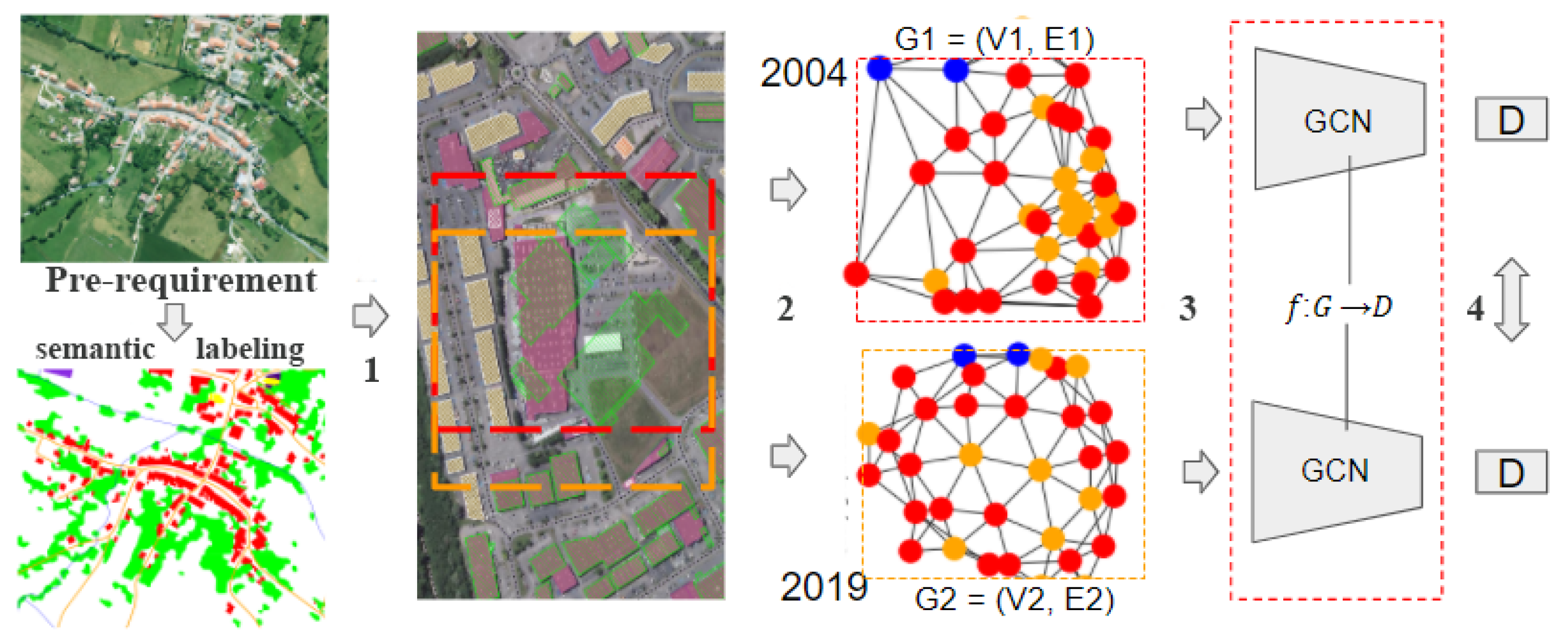
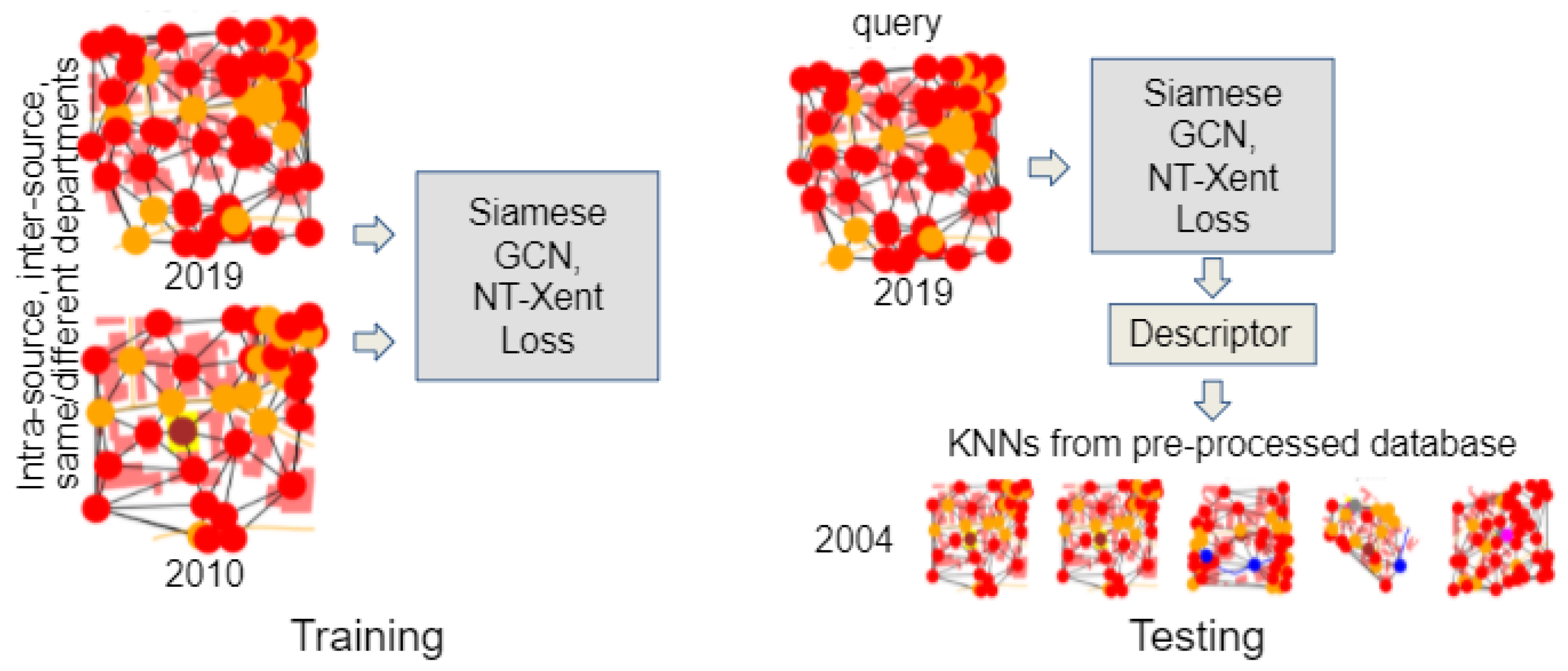
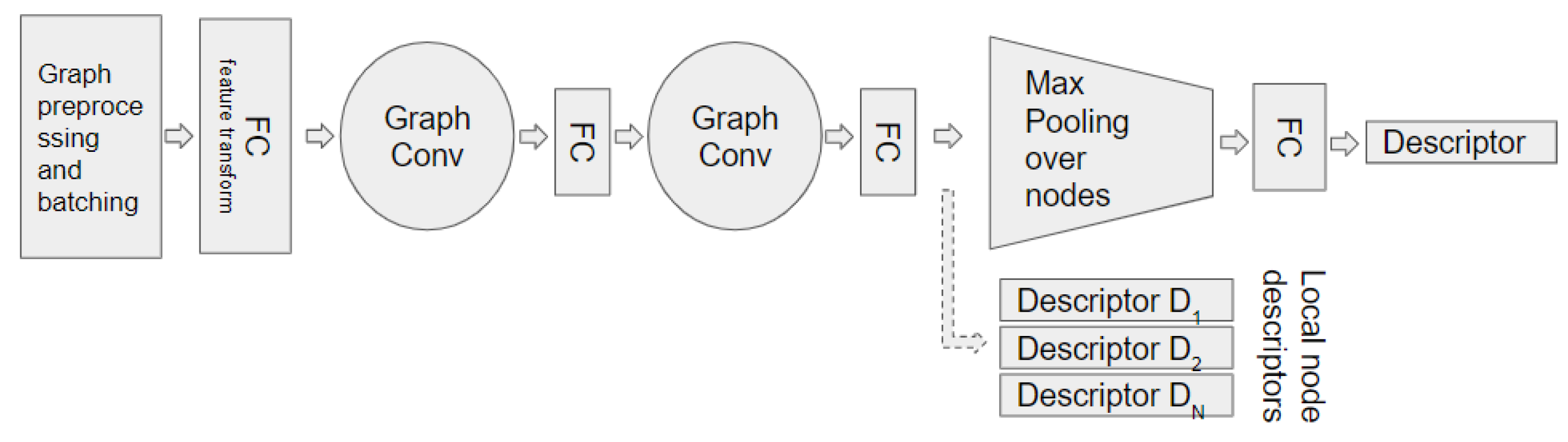
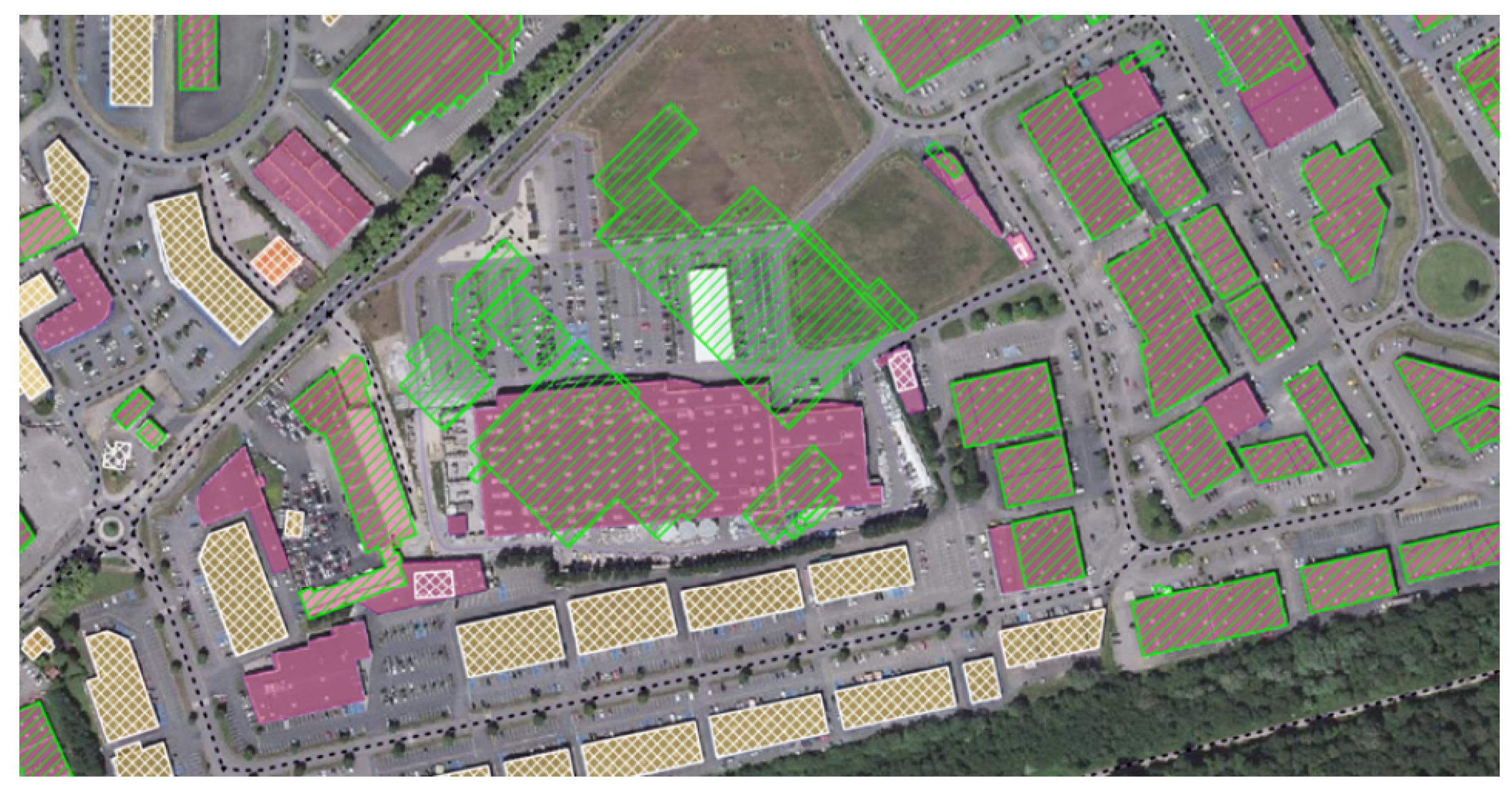
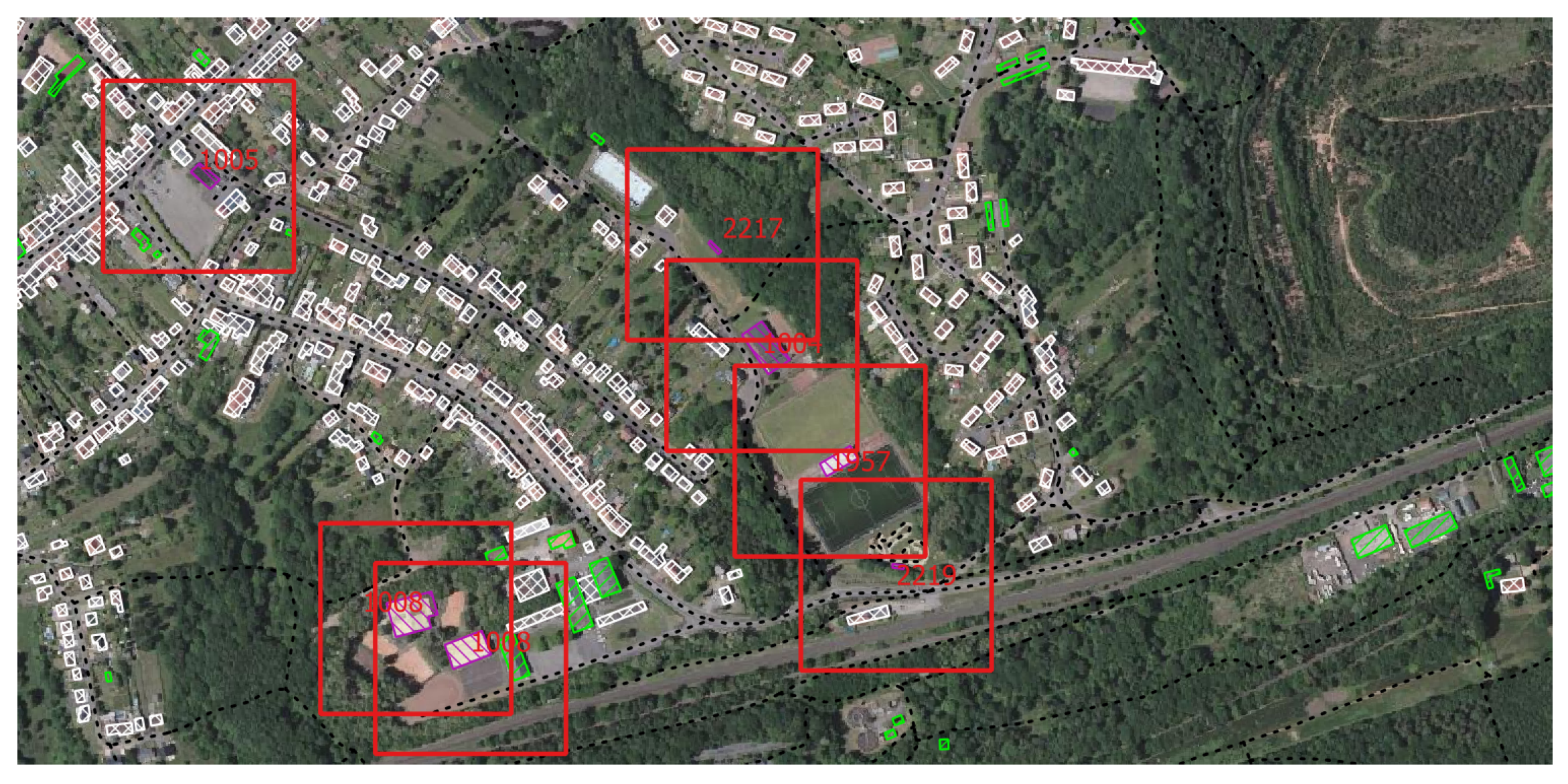
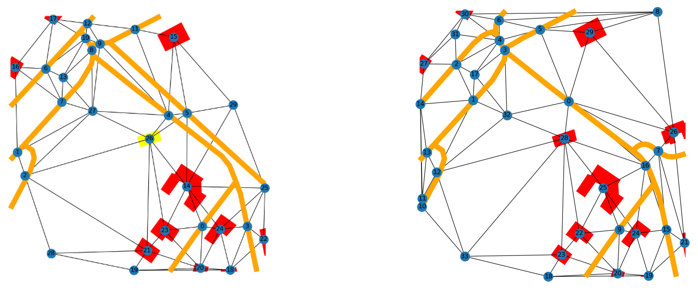
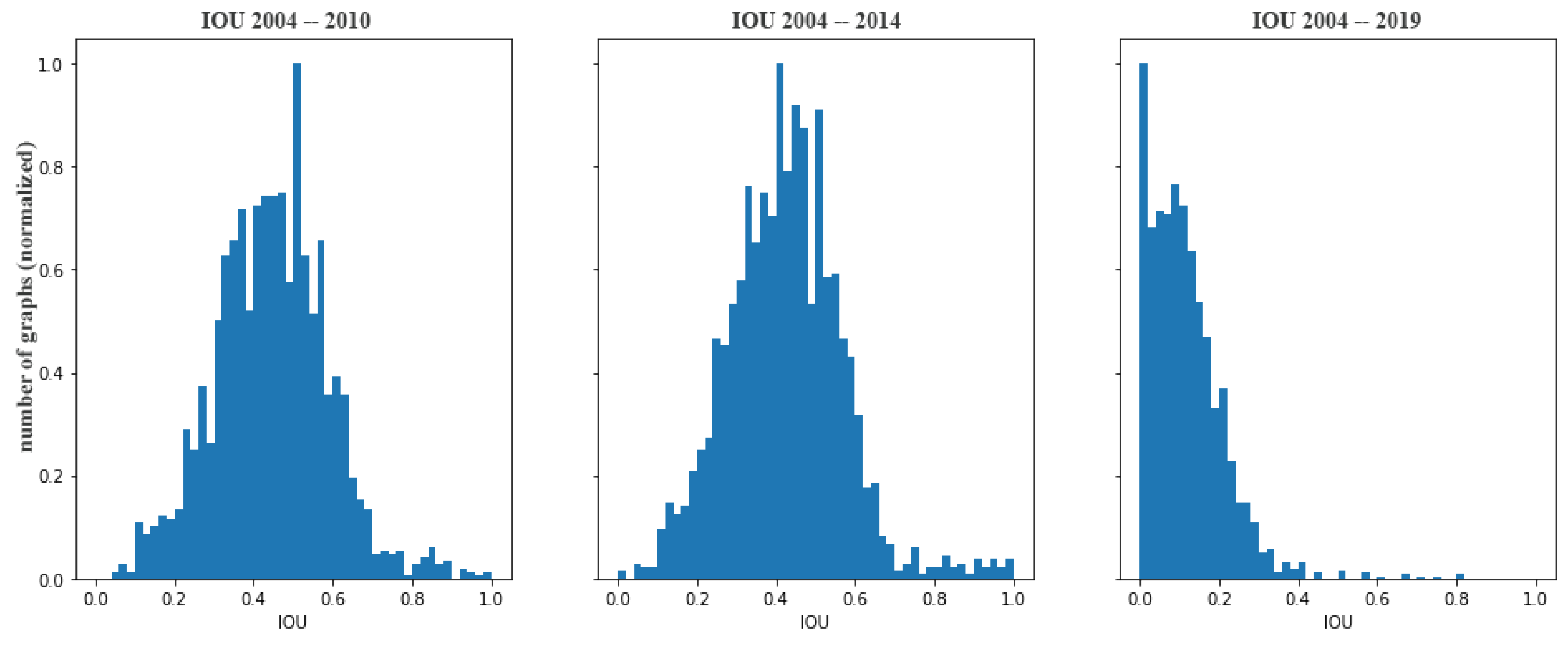
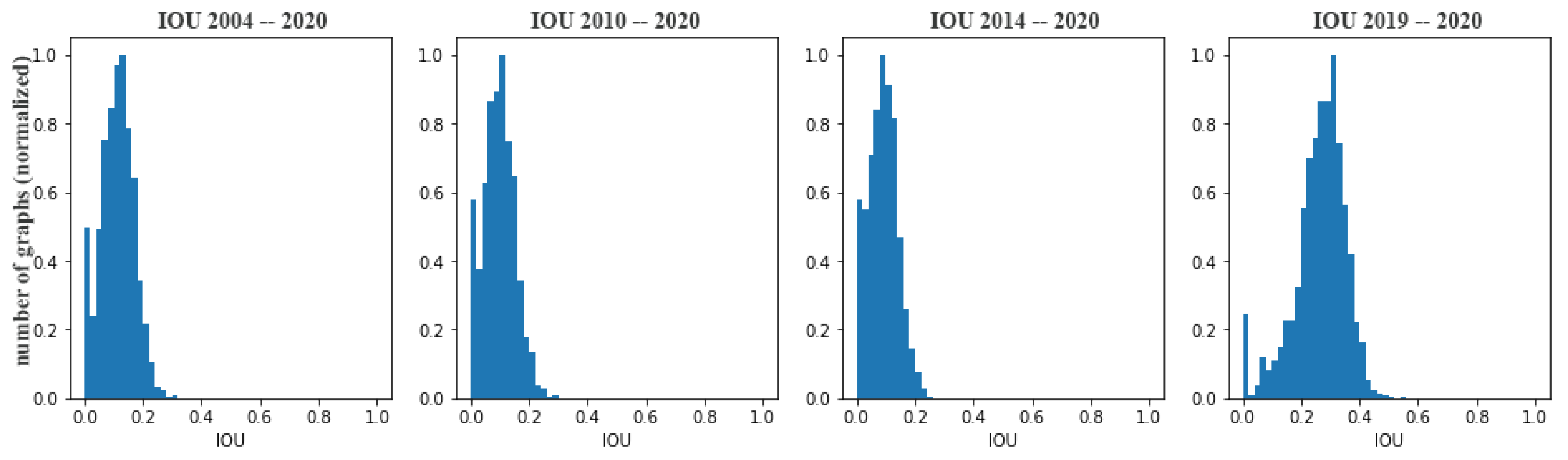
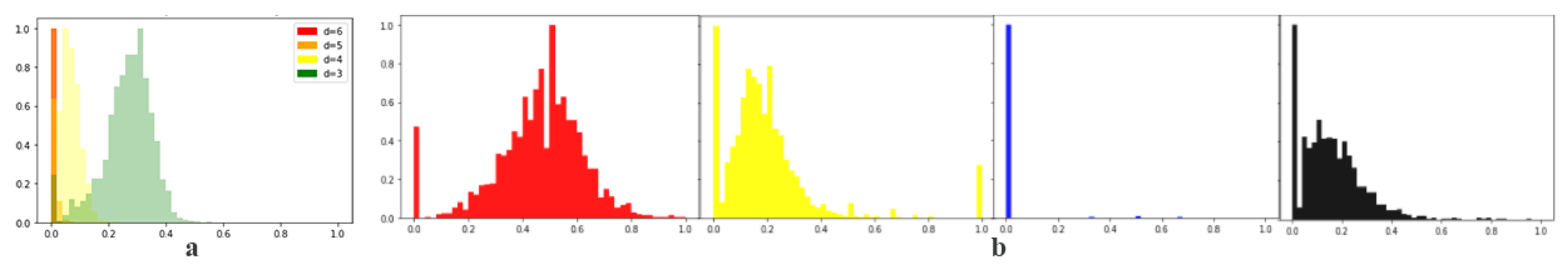
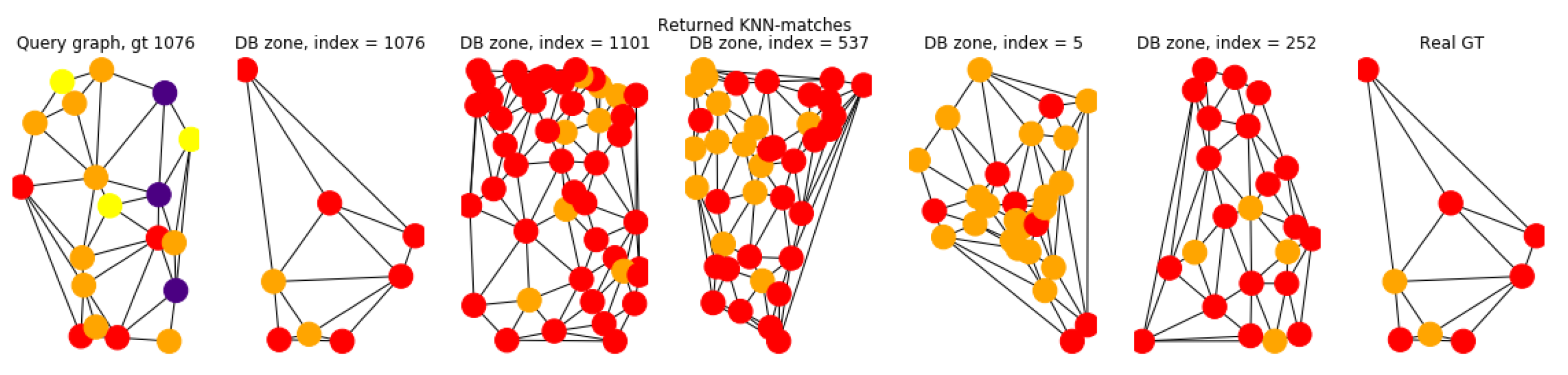
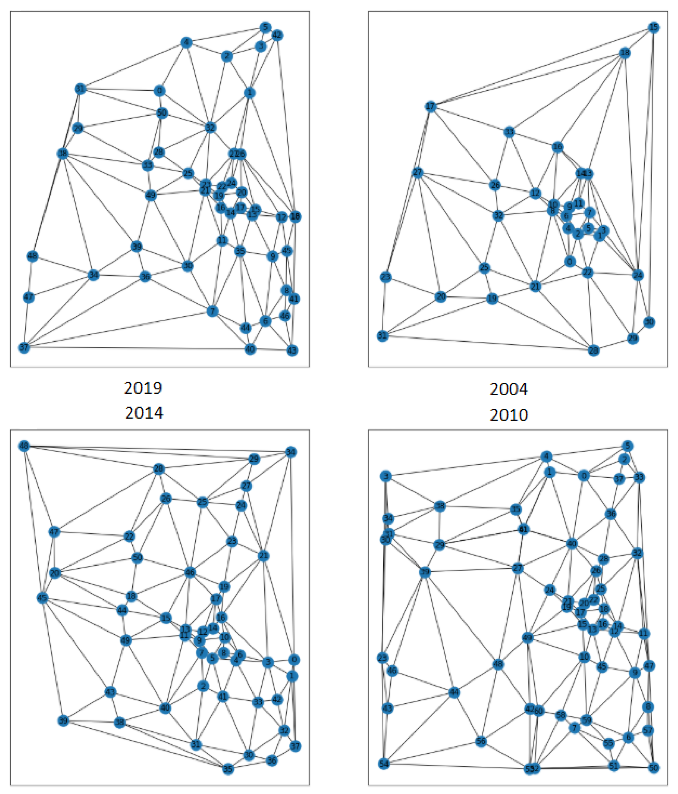
Table 1.
The characteristics of the proposed dataset for cross-time geographic area retrieval. Note that we mostly deal with single geographic area correspondence across years.
Table 1.
The characteristics of the proposed dataset for cross-time geographic area retrieval. Note that we mostly deal with single geographic area correspondence across years.
| Department | # Graphs | # Unique Areas | Years |
|---|---|---|---|
| Moselle | 2768 | 2298 | 2004, 10, 14, 19 |
| M-et-Moselle | 1968 | 1571 | 2004, 10, 14, 19 |
| Bas-Rhin | 2268 | 1863 | 2004, 10, 14, 19 |
| Côtes-d’Armor | 5029 | 5029 | 2004 |
| total | 12,033 | 10,761 | 4 time frames |
Table 2.
Single department statistics example.
| # nodes | # edges | Node Degree | ||
|---|---|---|---|---|
| db | Year | avrg, stnd, min, max | avrg, stnd, min, max | avrg, stnd, min, max |
| IGN | 2004 | 29.51, 15.16, 3, 91 | 76.78, 43.40, 3, 256 | 5.20, 1.25, 2, 12 |
| 2010 | 30.18, 15.39, 3, 92 | 78.73, 44.09, 3, 260 | 5.22, 1.25, 2, 11 | |
| 2014 | 65.83, 53.25, 3, 150 | 183.99, 156.97, 3, 280 | 5.59, 1.43, 2, 22 | |
| 2019 | 37.70, 19.59, 3, 125 | 100.62, 56.54, 3, 356 | 5.34, 1.26, 2, 14 | |
| OSM | 2020 | 33.24, 17.84, 3, 131 | 87.78, 51.51, 3, 378 | 5.28, 1.29, 2, 14 |
Table 3.
map@5 Faiss similarity search results, same source database with clutter graphs.
| Source | Query Year | db Year | map@5 | t per q (s) |
|---|---|---|---|---|
| same source | 2019 | 2004 | 0.827 | 0.05 |
| same source | 2014 | 2004 | 0.835 | 0.05 |
| same source | 2010 | 2004 | 0.924 | 0.04 |
| cross source | 2020 | 2019 | 0.80 | 0.04 |
| cross source | 2020 | 2014 | 0.11 | 0.04 |
| cross source | 2020 | 2010 | 0.04 | 0.04 |
| cross source | 2020 | 2004 | 0.07 | 0.04 |
Table 4.
No learning retrieval baseline using Faiss similarity search and modified node attributes.
| , Number of Decimals | with Noise, | ||||||
|---|---|---|---|---|---|---|---|
| Query Year | db Year | 1 | 2 | 3 | 0.1 | 0.01 | 0.001 |
| 2019 | 2004 | 0.007 | 0.254 | 0.825 | 0.009 | 0.126 | 0.647 |
| 2014 | 2004 | 0.007 | 0.261 | 0.835 | 0.010 | 0.170 | 0.778 |
| 2010 | 2004 | 0.011 | 0.455 | 0.924 | 0.011 | 0.224 | 0.902 |
Table 5.
Two scenarios used in our experiments.
| Scenario | Motivation | Separation Training/Testing | |
|---|---|---|---|
| 1 | cross-time learning approach | Train across time for two dates, and then retrive same regions dated from another year. | acquisition date |
| 2 | generalized learning approach | Test the generalizability of the method on departments unseen during training. | acquisition date, department |
Table 6.
The map@5 results for the global and local descriptors. Note that training and validation same-source training data do not contain clutter, but the testing data does. Cross-source test is performed without clutter data. Time is indicated in s.
Table 6.
The map@5 results for the global and local descriptors. Note that training and validation same-source training data do not contain clutter, but the testing data does. Cross-source test is performed without clutter data. Time is indicated in s.
| Global | Local | ||||||
|---|---|---|---|---|---|---|---|
| Query Year | db Year | Role | map@5 | t per q | map@5 | t per q | |
| same source | 2019 | 2010 | training | 0.660 | 0.017 | 0.303 | 0.880 |
| 2019 | 2014 | validation | 0.554 | 0.017 | 0.317 | 0.412 | |
| 2019 | 2004 | testing | 0.5522 | 0.017 | 0.371 | 1.14 | |
| 2010 | 2004 | testing | 0.684 | 0.019 | 0.638 | 0.97 | |
| cross source | 2020 | 2004 | testing | 0.056 | 0.01 | n/a | n/a |
| 2020 | 2010 | testing | 0.062 | 0.01 | n/a | n/a | |
| 2020 | 2014 | testing | 0.044 | 0.01 | n/a | n/a | |
| 2020 | 2019 | testing | 0.085 | 0.01 | n/a | n/a | |
Table 7.
The map@5 results for the single source database global and local descriptors with noise = 0.01.
Table 7.
The map@5 results for the single source database global and local descriptors with noise = 0.01.
| Global | Local | |||||
|---|---|---|---|---|---|---|
| Query Year | db Year | Role | map@5 | t per q | map@5 | t per q |
| 2019 | 2010 | training | 0.577 | 0.011 | 0.247 | 0.421 |
| 2019 | 2014 | validation | 0.483 | 0.011 | 0.314 | 0.517 |
| 2019 | 2004 | testing | 0.487 | 0.014 | 0.305 | 0.521 |
| 2010 | 2004 | testing | 0.628 | 0.014 | 0.578 | 0.314 |
Table 8.
The map@5 results for the global and local descriptors, cross-department learning.
| Global | Local | |||||
|---|---|---|---|---|---|---|
| Query Year | db Year | Role | map@5 | t per q | map@5 | t per q |
| 2019 | 2004 | training | 0.538 | 0.01 | 0.399 | 0.6 |
| 2019 | 2004 | testing | 0.576 | 0.003 | 0.371 | 0.2 |
Table 9.
The map@5 results for the global and local descriptors, cross-year correspondence learning, cross-source data.
Table 9.
The map@5 results for the global and local descriptors, cross-year correspondence learning, cross-source data.
| Global | Local | |||||
|---|---|---|---|---|---|---|
| Query Year | db Year | Role | map@5 | t per q | map@5 | t per q |
| 2020 | 2004 | training | 0.29 | 0.02 | 0.07 | 0.23 |
| 2020 | 2019 | validating | 0.33 | 0.02 | 0.18 | 0.27 |
| 2020 | 2014 | testing | 0.15 | 0.02 | 0.44 | 0.30 |
| 2020 | 2010 | testing | 0.17 | 0.02 | 0.44 | 0.23 |
Table 10.
The map@5 results for the global and local descriptors, cross-department learning and testing, cross-source data.
Table 10.
The map@5 results for the global and local descriptors, cross-department learning and testing, cross-source data.
| Global | Local | ||||||
|---|---|---|---|---|---|---|---|
| Department | Query Year | db Year | Role | map@5 | t per q | map@5 | t per q |
| Moselle | 2020 | 2019 | training | 0.61 | 0.02 | 0.22 | 0.15 |
| M-and-Moselle | 2020 | 2019 | testing | 0.513 | 0.02 | 0.23 | 0.11 |
| 2020 | 2004 | testing | 0.128 | 0.02 | 0.005 | 0.11 | |
Publisher’s Note: MDPI stays neutral with regard to jurisdictional claims in published maps and institutional affiliations. |
© 2022 by the authors. Licensee MDPI, Basel, Switzerland. This article is an open access article distributed under the terms and conditions of the Creative Commons Attribution (CC BY) license (https://creativecommons.org/licenses/by/4.0/).
Share and Cite
MDPI and ACS Style
Khokhlova, M.; Abadie, N.; Gouet-Brunet, V.; Chen, L. GisGCN: A Visual Graph-Based Framework to Match Geographical Areas through Time. ISPRS Int. J. Geo-Inf. 2022, 11, 97. https://doi.org/10.3390/ijgi11020097
AMA Style
Khokhlova M, Abadie N, Gouet-Brunet V, Chen L. GisGCN: A Visual Graph-Based Framework to Match Geographical Areas through Time. ISPRS International Journal of Geo-Information. 2022; 11(2):97. https://doi.org/10.3390/ijgi11020097
Chicago/Turabian StyleKhokhlova, Margarita, Nathalie Abadie, Valérie Gouet-Brunet, and Liming Chen. 2022. "GisGCN: A Visual Graph-Based Framework to Match Geographical Areas through Time" ISPRS International Journal of Geo-Information 11, no. 2: 97. https://doi.org/10.3390/ijgi11020097
Note that from the first issue of 2016, this journal uses article numbers instead of page numbers. See further details here.