Predicting Electric Vehicle Charging Station Availability Using Ensemble Machine Learning

Abstract

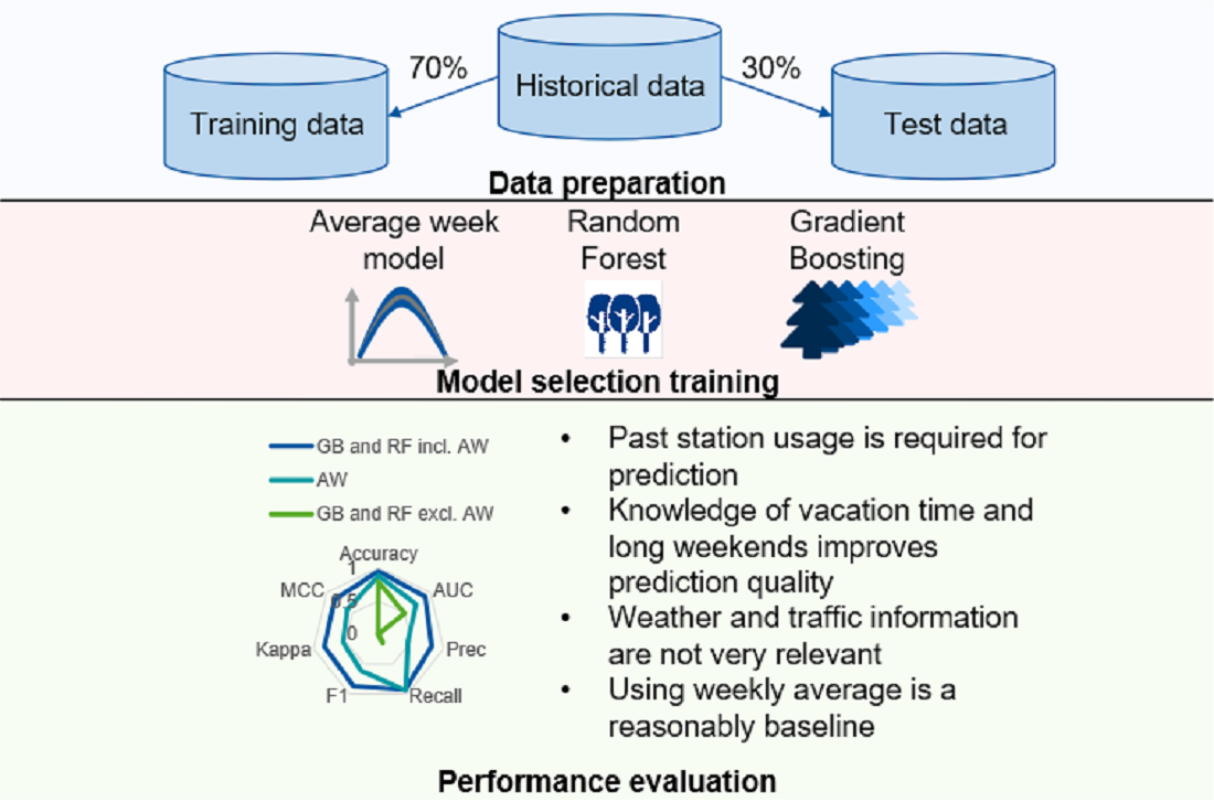
Electric vehicles may reduce greenhouse gas emissions from individual mobility. Due to the long charging times, accurate planning is necessary, for which the availability of charging infrastructure must be known. In this paper, we show how the occupation status of charging infrastructure can be predicted for the next day using machine learning models— Gradient Boosting Classifier and Random Forest Classifier. Since both are ensemble models, binary training data (occupied vs. available) can be used to provide a certainty measure for predictions. The prediction may be used to adapt prices in a high-load scenario, predict grid stress, or forecast available power for smart or bidirectional charging. The models were chosen based on an evaluation of 13 different, typically used machine learning models. We show that it is necessary to know past charging station usage in order to predict future usage. Other features such as traffic density or weather have a limited effect. We show that a Gradient Boosting Classifier achieves 94.8% accuracy and a Matthews correlation coefficient of 0.838, making ensemble models a suitable tool. We further demonstrate how a model trained on binary data can perform non-binary predictions to give predictions in the categories “low likelihood” to “high likelihood”.

1. Introduction

Electric vehicles (EVs) are generally seen as a viable path towards reducing CO2 emissions from mobility. In the context of this paper, we focus on battery electric or plug-in cars. These vehicles store (some of) the energy required for propulsion and auxiliary in an internal traction battery that is recharged through an electricity grid connection. While the share of EVs in car sales might have been considered negligible in the past several years, this cannot be considered true anymore—globally and in Germany. Globally, China had been market leader for several years in terms of absolute numbers, with annual sales exceeding one million vehicles for the first time in 2018 [1]. Likely due to a reduction in subsidy, the local market lost some of its dynamic growth recently. European governments such as Germany, France, Italy, and some others in turn have increased subsidies and other regulatory measures significantly [2]. In combination with the stricter EU fleet emission targets, Europe is now the globally leading market for EV sales, with 747,000 battery electric vehicles and 625,000 plug-in hybrid electric vehicles sold in 2021 alone [1]. Germany has been spearheading this development, with up to EUR 9000 in subsidies for new EVs, the worldwide fourth-highest share of battery and plug-in electric vehicles worldwide, and the highest absolute numbers in Europe [1]. The governmental goal of a cumulative sale of one million vehicles was reached, with a slight delay of 8 months, in August 2021 [3]. These trends and developments clearly show that the market is picking up pace. Using the typically used diffusion of innovation curve, one can state that the market is moving away from early innovators and is entering the early adopters or even early majority stage instead [4].

To achieve the widespread adoption of EVs, it is essential to have sufficient public charging infrastructure (CI) available such that users are able to comfortably and quickly recharge their EVs [5,6,7]. Currently, EV drivers in Germany are billed for CI usage at a fixed price per kWh and sometimes additionally for parking time. The situation may be different elsewhere, but generally does not vary significantly. Fixed price mechanisms lead to the highly inhomogeneous usage of CI, with occupation rates differing widely between day and night as well as between weekdays [8]. This is clearly not ideal as it leads to potentially avoidable charging hotspots where little to no CI is available. Some EVs may, however, already have a high state of charge and only recharge because the opportunity arises, while others urgently require recharging. During these shortages, drivers with a relatively high battery state of charge should be incentivised to give up their recharging opportunity for somebody with a more urgent recharging need. Implementing a system that globally optimises CI allocation is, however, not feasible for public CI as these devices should be easily accessible.

An alternative solution to the aforementioned problem is to vary prices. With current vehicle batteries covering 300 km and more of range [9], recharging has to happen only occasionally if persons drive 39 km/day on average in Germany [10,11]. If such persons were price-sensitive, it would be possible to incentivise them to charge when sufficient CI is available and, hence, indirectly support the grid load or capacity, respectively. This is the goal of the project BeNutz LaSA [12], in which the authors together with partner organisations implement such a price-based incentive mechanism in Germany.

Charging typically takes hours, especially at slower AC stations, and it is not feasible to force users to stop their charging spontaneously. If a shortage of CI occurs, we therefore cannot simply reduce the current occupation. For this reason, the authors attempt to predict CI usage with the goal of adapting prices already before a hotspot materialises. In this context, a good prediction is one that accurately predicts the occupation for as many stations as possible. The methodologies presented to achieve such a prediction can be used worldwide and are evaluated with real-world charging data in the use case of Germany.

The main aim of this paper is consequently to derive and evaluate methods to predict the status of many stations as accurately as possible and to give a measure of certainty on a station-by-station level. The paper is structured as follows: in the next Section 1.1 and Section 1.2, the current literature on the issue is summarised. The following section, “Materials”, contains all data sources used in this work. Section 3, “Methods”, outlines all methods applied on the data. The results are presented in Section 4, “Results”. The discussion and conclusions are provided in Section 5 and Section 6, respectively. The back matter contains, in order of appearance, the acknowledgements, funding information, author contributions, data availability, software availability, the ethics statement, and lists of tables and figures.

1.1. Literature Review

Predicting the usage of CI is a much-discussed topic in the literature. One strand of literature focuses on which locations are sensible ones for the construction of CI [13,14,15,16], some with a focus on when future stations are likely to be used [17]. These models tend to have a longer-term focus and are not very relevant to the work done in this paper, where the goal is to predict short-term charging hotspots for the next day(s).

In the field of predicting the usage of individual stations for the short-term future, much less work has been published [18,19,20,21]. These authors attempt to generate a time series prediction for specific charging stations. The works, however, focus on very specific sites, such as a university campus [18], workplace charging [19], or EV taxis in the metropolitan area of Shenzhen [20], and therefore cannot serve as a model for a national scope, as done in this paper. Given the small geographic area, employing the used models may not be suitable for our purposes, as a risk of overfitting exists. A key reason for this is that models sometimes require specific conditions to be true to be applicable. Simple time series models focusing on a few points, such as done by Majidpur [18], fail if the patterns become highly irregular and cannot absorb the depth of information that our dataset contains. The models and methods, however, do provide a starting point for this work as they are a mix of classical statistical methods and machine-learning-based ideas.

Almaghrebi et al. [22] focus on a slightly different challenge. They attempt to predict energy requirements once a charging session has started given past CI usage data. They employ four models, namely a linear model, a gradient booster, a random forest, and a support vector machine. These concepts are also looked at in this paper. Frendo et al. [23] take this process one step further and examine the behaviour of an entire fleet and additionally provide an extensive literature review in their particular field. The complimentary challenge of trying to predict energy consumption while the vehicle is on the road is also being tackled using very similar methods [24,25].

An analogous problem that has received much more attention in the past is the prediction of the availability of bicycles at public bicycle sharing stations [26,27,28,29,30,31,32,33,34,35]. The problems are comparable since there are a number of spots that can either be occupied or not and it is relevant to determine when stations are out of bicycles to rent. The employed tools are quite similar to the ones used for CSs and include statistical models or machine learning models. Examples for the former are a generalised extreme value count model [28], dynamic linear models [29], generalised additive models [30], autoregressive, or autoregressive, integrating, moving average models (ARIMA) [26]. These models can typically be employed when usage patterns are fairly regular, particularly for the latter two. This requires the observed number of stations to be sufficiently aggregated such that random fluctuations do not have a major impact. In the context of this paper, the aggregation unit is the individual CS, with the corresponding high noise making such tools unsuitable. A selection of employed machine learning models includes random forest models [26], deep learning models [27], k-means clustering [31,32], or, less frequently, models such as the averaged one dependence estimators with subsumption resolution model [33]. Most of these models are in fact quite useful for our purpose as well and have been investigated. Deep learning, such as done by Yoshida et al. [27], however, requires that more input variables are available per decision than is possible in this paper. In other words, a CS history is not relevant for future events apart from the average weekly usage. We therefore do not consider deep learning models. Next to these time series models, it is also possible to use more holistic models, such as multi-agent systems [34] or flow-based models [35].

Looking at the three outlined categories, we can try to understand the applicability of the used methods for the purpose of CS availability prediction. In general, there are no models that are being used much more frequently than others, but, rather, models are selected to fulfil a specific purpose in each publication. The only important trend that we saw in researching the literature was that the easier-to-implement, standard models are more popular than their more complicated counterparts are. This can presumably be linked to the fact that most researchers come from the technical domain and not so much from the data science domain and therefore rely on existing libraries.

The statistical models can only be used on a large scale when trying to understand and predict trends involving hundreds of CSs. The reason for this is that the usage patterns at individual CSs are highly inhomogeneous and often do not follow a regular pattern consistently, as the standard deviations calculated in our previous work show [8]. An ARIMA model, for instance, would see far too irregular usage in the weeks before the predicted hour to provide any useful prediction.

The machine learning models used are very similar to the ones used in the prediction of CS availability. A more detailed analysis of which of these models is suitable follows later in the paper.

The last category of more holistic models is very challenging to create for cars. The reason for this is that cars move much further and for much more diverse reasons. Bicycle rides are typically limited to a few kilometres and there is no option to transport heavy goods on bikes. These two effects automatically limit the diversity of possible trip purposes and therefore make it much easier to develop models of the vehicles’ movement. In contrast, the movement of EVs is far more diverse. An additional challenge is that public bicycle operators are able to track where the bikes are going, but no such data are available for (private) cars to protect the privacy of drivers.

1.2. Improvements of This Paper in the Context of the Literature

This paper uses similar machine learning and statistical tools as some previous work has already done [18,19,20,21] and thereby verifies the applicability of these tools. Our key contribution and thereby advancement compared to the current state of the art is that we are able to include a much broader geographic scope for our time series prediction as compared to previous publications. This Germany-wide approach allows us to ensure that overfitting is limited given the diverse geographies and characteristics, ranging from small villages all the way to larger metropolitan areas such as Munich, Berlin, or Hamburg. This wide geographical scope further ensures that the results are representative at least for European countries and possibly even for other geographies. We further advance the literature by clearly showing which models were used, why they were used, and how they were tuned. This will help fellow researchers in deciding which model to use in their own applications.

2. Materials

In this paper, several data sources are used. These are explained in the following subsections. All datasets are geographically referenced time series datasets that need to be merged into one single input table. Merging is done based on geographical reference and time.

While outlining the data used, it is also important to state which data were not used and why. This paper intentionally does not employ datasets that describe the static environment of the CS. Examples of such sets could be OpenStreetMaps points of interest, population density, number of registered cars, etc. While these factors are certainly important in understanding why and how CSs are used, this was not of relevance in this paper. The reason is that the past CS usage data provide a much better picture of usage patterns than environmental factors. Given that we assume there to be a usage history for each station, it is consequently superfluous to describe the environment and we focus solely on features changing quickly with time.

2.1. 2019 vs. 2021 Dataset

In this work, we define two datasets, one starting in 2019 and one starting in 2021. The reason for this difference is that traffic data are available only from 2021 onwards, while CS occupation was available from 2019 onwards. A benefit of this split is that we can observe whether longer or shorter training data are preferable. The split between the two datasets was performed across all datasets listed in the following.

2.2. CS Usage Data

In the context of the project BeNutz LaSA [12], the ISEA institute has received the CS occupation from the industry partners SMART/LAB and Hubject. The dataset can be converted into CS hours, where each data point describes the status of a CS for a given hour. This hourly status was defined by dividing the occupied time by one hour and the number of EVSEs at a specific CS, as shown in the below equation.

$$occupation=\frac{T_{occupied}}{1h\cdot {\#}_{EVSEs}}$$

(1)

where $T_{occupied}$ is the sum of all time that vehicles spent at the CS in the given hour. Multiple vehicles can result in $T_{occupied}$ becoming larger than 1. The variable ${\#}_{EVSEs}$ is the number of EVSEs at the CS. A typical station with two EVSEs would consequently have an occupation of 50% if one of the two EVSEs were fully occupied during the hour while the other one remained available for customers, both were occupied for half an hour, or any possibility in between these two options.

The total number of data points was around 90 million, out of which 12% had missing information. The time period analysed was approximately two years and nine months from 1 January 2019 to 12 September 2021. Reasons for missing information could be that the station was built during the time analysed and, therefore, historical data were unavailable earlier, the station was a test station, no matching weather station or area for traffic analysis could be found, or the station’s given latitude and longitude was outside of the boundaries of a state. For this paper, the aspects of the data that were used were:

• Status changes of the EVSEs as defined by the Open Charge Point Protocol [36];
• Location of the charging infrastructure;
• Grouping of EVSEs into charging stations.

2.3. Public Holidays and School Holidays

Public holidays were retrieved using the Python library holidays [37]. The library allows us to check whether a date is a public holiday in countries and in the states of these countries. In this work, the public holidays on the level of German states are considered. Public holidays sometimes create long weekends, which are frequently used for short trips. This increased mobility was assumed to have an impact on charging station usage, which is why long weekends were also detected by checking whether public holidays were either directly adjacent to a weekend or with only a single day in between.

School holidays were retrieved from Ferienwiki.de [38]. The website provides iCal files containing school holidays. The school holidays are defined on a state level in Germany and can be quite different in terms of when they occur and how long they are. No correction is made in this paper for cases where stations are near state borders since it is challenging to define how the effect should be quantified.

2.4. Weather Data

Precipitation and temperature time series were downloaded from the open data portal of the German weather service, DWD [39,40]. The data comprise time series measured at 468 weather stations. Temperatures were recorded as the average temperature over one hour in °C and precipitation in $\frac{mm}{h}$. Stations at an altitude above 1000 m were filtered out since the weather service operates stations on mountaintops, which would clearly not be representative for the weather situation where people live.

All weather datasets further contain a measure of accuracy and an indication of the equipment used to obtain said values. Given that the used data were quite recent, this information was of no relevance in this project since all stations have been operating with high-quality equipment over the last few years. Inaccuracies due to imprecise equipment occurred in the beginning of the time series, which, for many stations, was in the 20th century.

2.5. Traffic Data

Traffic data were purchased from ADAC Service GmbH [41] for this project. ADAC has trackers in over 300,000 vehicles in Germany and receives their position, velocity, and several other values. The data split Germany into rectangles of approximately 1.8 × 1.8 km and are available at an hourly resolution. For each such rectangle, the dataset contains the number of fleet vehicles that were in the rectangle during this hour. An example of the data can be found in

Table 1. Sample of data obtained from ADAC.

Tile x-Coordinate	Tile y-Coordinate	Date and Time	Number of Vehicles
8653	5276	2021-01-05 06:00	353
8662	5293	2021-01-05 08:00	214
8660	5288	2021-01-08 01:00	166

.

While the number of vehicles is not the traffic intensity itself, the monitored fleet is large enough that it can be understood as a proxy for traffic intensity. The recorded data have been provided from the start of 2021 onwards and predictions are delivered on a daily basis. In this work, only the recorded past has been used.

3. Methods

This chapter describes the methodology used in this paper. The different data sources listed in the “Materials” section were matched as outlined in “Data Merging”. The resulting full datasets were processed as explained in “Data Preprocessing”. The final dataset was then fed into several prediction models, which are given in “Chosen Prediction Models”. The evaluation steps relevant for discussion are not outlined in the methodology section since common metrics were used.

3.1. Data Merging

Data matching was performed based on the location of the charging station. For weather data, each charging station was matched with the nearest available weather station using cKDTree from scipy.spatial [42]. Weather stations were marked as usable if data were recorded for the time period observed in this paper and if they were located at a height of less than 1 km. The latter criterion was introduced to filter weather stations located on mountaintops, such as the one on top of the mountain Zugspitze.

For spatial properties such as holidays and vacation periods that relate to entire states, charging stations were matched to the state that they were in using the Geospatial Data Abstraction Library in combination with its Python bindings.

3.2. Data Preprocessing

Models learning from large datasets can be subject to overfitting, where random noise in the training set is interpreted as an actual signal that the models interpret as significant. For the data discussed in this paper, the risk of overfitting is particularly prominent for weather data. The reason for this is that human behaviour does change with the weather but is generally agnostic to minor changes. A person would, for instance, drive to a nearby forest for a hike if it were warm and dry, but would not care about exact values for precipitation or temperature. To adjust for these somewhat coarser categories, precipitation was split into three levels of rain, which more or less corresponded to no rain, little rain, and heavy rain, as shown in Equation (2). These levels were chosen based on the analysis of the dataset used in our previous publication [8].

$$prec=\{\begin{array}{cc}0& if pre{c}_{full}=0\\ 1& if 0<pre{c}_{full}<4\\ 4& if pre{c}_{full}\le 4\end{array}$$

(2)

where $pre{c}_{full}$ are the measured precipitation values obtained from the weather stations in $\frac{mm}{h}$ on the right-hand side. The variable $prec$ in turn is the categorised precipitation.

To avoid overfitting for temperature, the recorded temperature was rounded to the nearest multiple of five since this is sufficiently granular to correspond with the human sensation of temperature but simultaneously coarse enough to avoid overfitting.

For the traffic data, we calculated how many vehicles were in a square relative to the square’s average usage to provide a measure of how much the current traffic deviated from the traffic that the area would normally experience.

All datasets used in this work are time series. The next step of data preprocessing was consequently to align the various datasets along the time axis. This was done for each CS separately. An example of such a dataset can be seen in

Table 2. Example of the merged dataset.

Occupation	Vacation	Long Weekend	Temperature	Precipitation	Number of Vehicles	Relative # Vehicles	Weekday	Hour
[0,1]	TRUE/FALSE	TRUE/FALSE	°C	$\frac{mm}{h}$	#	%	[0–6]	[0–23]
0.000	1	0	15	1	166	150%	1	14
0.667	1	0	15	0	130	83%	3	0
0.932	0	1	5	0	202	216%	0	12

.

3.2.1. Feature Categorisation

While the calculated occupation, in theory, is a continuous variable and regression models could be employed to predict the occupation numerically, this is neither achievable nor desirable. The non-achievability stems from the fact that the provided features do not carry sufficient information to explain minor differences such as a vehicle leaving a few minutes earlier or later, which would in turn change the occupation. It is also not desirable since the goal of the project is to create a more human-readable output. The resulting occupation probabilities would likely be very confusing for users, particularly when compared to the chosen categories “very low” to “very high”.

It was consequently necessary to create a categorisation of the occupation as a feature. This was done in two ways, which we will refer to as binary and categorised.

The binary classification, as the name already suggests, is a classification into binary values. We chose to set a boundary at 50%, as shown in Equation (3). The boundary was chosen since a 50% occupation means that only one EVSE was available on average at a typical CS with two EVSEs. A newly arriving vehicle would consequently cause the full usage of the station and no additional customers could be served. Additionally, virtually all CSs have an even number of EVSEs, leading to a good fit when taking half of 100%.

$$binary=\{\begin{array}{cc}TRUE& if occupation\ge 50\%\\ FALSE& otherwise\end{array}$$

(3)

where $occupation$ has been defined in Equation (1).

The categorised classification is meant for users of CI. The goal is to provide a human-readable classification in the categories “very low” ($vl$), “low” ($l$), “medium” ($m$), “high” ($h$), and “very high” ($vh$). These five categories are defined by occupation as well, as shown in Equation (4).

$$categorised=\{\begin{array}{cc}vh& if occupation\ge 40\%\\ h& if 30\%\ge occupation<40\%\\ m& if 20\%\ge occupation<30\%\\ l& if 10\%\ge occupation<20\%\\ vl& otherwise\end{array}$$

(4)

where $occupation$ has been defined in Equation (1).

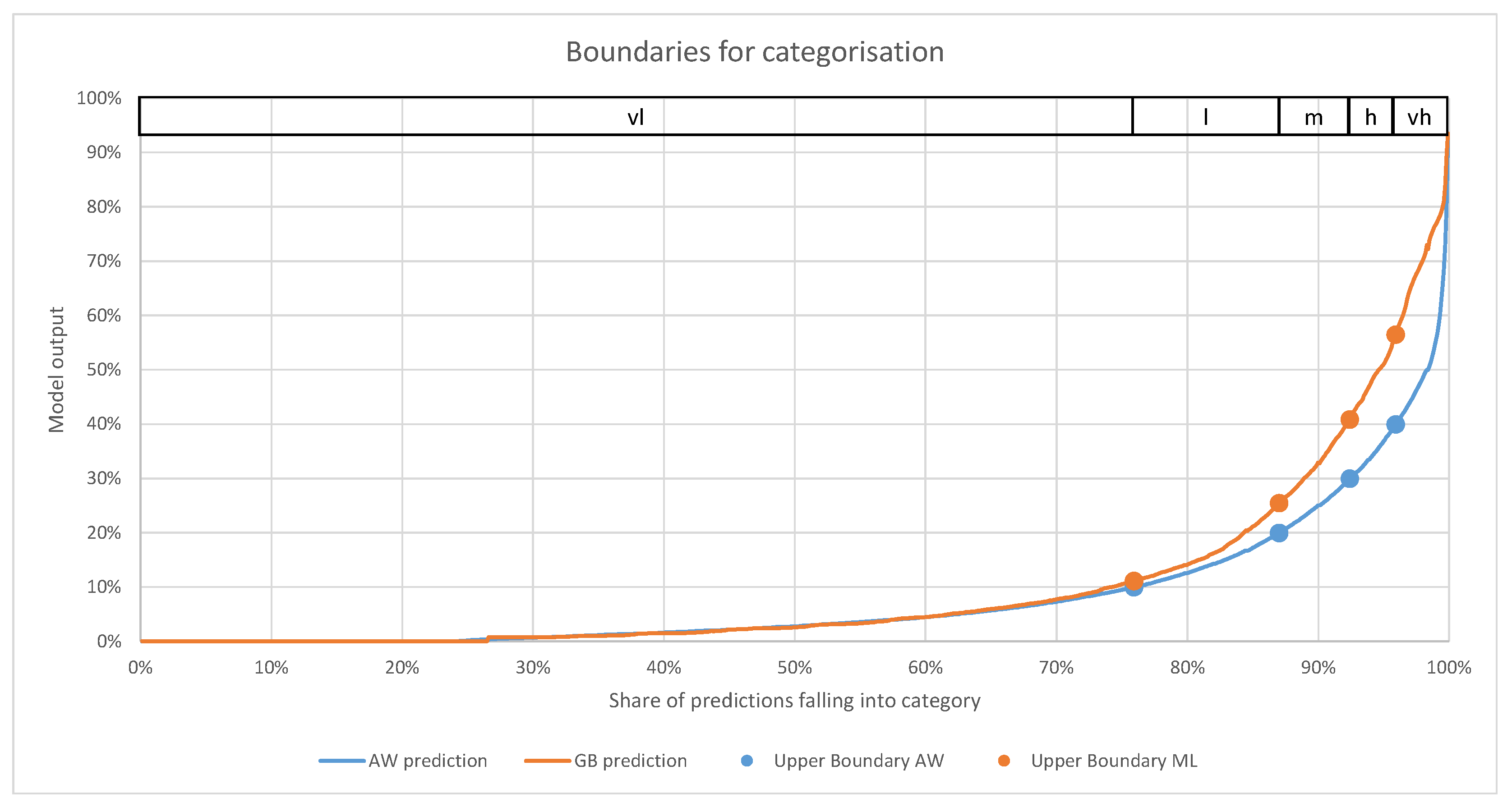
This classification was chosen based on an analysis of which categories appear how frequently while simultaneously using easy-to-remember boundaries. Different categorisations are certainly possible and will be explored in our future works. The given one is arbitrary to an extent. The results of GB and RF cannot be used directly for the categorisation since the output probability is defined as the probability that the station is occupied up to 50%. This was resolved by running many test predictions and creating a translation function. This function is simply a set of new boundaries that were chosen such that the size of the predicted groups is equal to the sizes when using AW on a set of test predictions. The boundaries are given in Equation (5) and the concept is visualised in Figure 1. As shown, the boundaries of the occupation are translated into group sizes by checking which x-value corresponds to the given y-values. These x-values were then kept and the corresponding y-values of the test predictions were chosen. The process was executed only for GB, but, as will be seen later, the prediction values were very close for both models and the same categorisation boundaries may be used.

$$ccategorised=\begin{array}{c}\\ \{\begin{array}{cc}vh& if prediction\ge 56.5\%\\ h& if 40.9\%\ge prediction<56.5\%\\ m& if 25.5\%\ge prediction<40.9\%\\ l& if 11.2\%\ge prediction<25.5\%\\ vl& otherwise\end{array}\\ \end{array}$$

(5)

where $prediction$ is the output value generated by the machine learning models.

3.2.2. Train–Test Split

For the evaluation of machine learning models, one typically splits the data into a training and a test set. This was done in this work as well. Test feature–label combinations were randomly drawn from the dataset until 30% of the dataset was used. The remaining 70% were used for training. Note that this split consequently does not orient itself along a time axis and we therefore do not predict the last 30% in terms of time. This was done since models will be retrained regularly in real-world application and, given the highly dynamic market development, it is not sensible to use months-old models.

3.3. Model Selection

The proper analysis of the suitability of a model requires significant computational and time resources. To gain an overview of which model is suitable for the task and how the different models compare, a comparison was performed using the function classification.compare_models() of the library PyCaret [43]. The library wraps other machine learning libraries such as sklearn [44] and calls the most frequently used models using their standard settings. The models are consequently not optimised for their final task and overfitting might be an issue in certain cases. Results should therefore be understood as indicative and must be confirmed with properly tuned models, which was performed in the second part of this paper.

The goal of performing the model comparison was to evaluate whether the models outlined in the Section 3.4 “Chosen Prediction Models” were comparable in performance to other models. The choice for the actual implementation was, however, limited to models providing an uncertainty measure since the goal is not to perform binary prediction as accurately as possible but rather to later perform categorised prediction. Further, note that the average week model does not appear in the overview provided by PyCaret. It was added by us due to its low complexity and since it is easy to understand for end users and system administrators. Deterministic models were not evaluated since it could be shown in previous work that these are not sufficiently accurate.

3.4. Chosen Prediction Models

In this work, several prediction methods are tested and compared with each other. The Random Forest Classifier (RF) and Gradient Boosting Classifier (GB) were selected as typically used ensemble models and because of their high prediction performance, as shown in

Table 3. Result of PyCaret’s model comparison using 10 million randomly sampled rows of the 2021 training set. The best score per metric is marked in boldface. Accuracy: 94.35%, AUC: 0.9765, Precision 91.46%, F1: 0.8591, Kappa: 0.8239, MCC: 0.8263.

Model	Accuracy	AUC	Recall	Prec.	F1	Kappa	MCC
Light Gradient Boosting Machine	0.9435	0.9765	0.8099	0.9146	0.8591	0.8239	0.8263
Gradient Boosting Classifier	0.9432	0.9747	0.811	0.9121	0.8586	0.8232	0.8254
Ada Boost Classifier	0.9431	0.9697	0.8093	0.9132	0.8581	0.8227	0.825
Ridge Classifier	0.9429	0	0.8181	0.9043	0.8591	0.8234	0.825
Linear Discriminant Analysis	0.9421	0.9688	0.8244	0.8949	0.8582	0.8219	0.823
Logistic Regression	0.9407	0.9682	0.8297	0.8841	0.856	0.8187	0.8194
Random Forest Classifier	0.9404	0.9702	0.81	0.8998	0.8526	0.8154	0.8172
Extra Trees Classifier	0.9368	0.9634	0.8095	0.8834	0.8448	0.8052	0.8064
SVM— Linear Kernel	0.9248	0	0.797	0.8482	0.8181	0.771	0.7742
Naive Bayes	0.9218	0.9529	0.843	0.8001	0.821	0.7711	0.7715
Decision Tree Classifier	0.914	0.8755	0.7952	0.7994	0.7973	0.7428	0.7428
K Neighbours Classifier	0.8284	0.7782	0.3238	0.712	0.4451	0.3601	0.3993
Quadratic Discriminant Analysis	0.6291	0.4999	0.2752	0.212	0.2047	−0.0001	−0.0003

. Additionally, the average week model (AW) was added as a reference since, nowadays, many websites use this metric to inform customers about when to expect how many other customers. The chosen models are described in detail in the respective subsections. GB and RF were both trained and evaluated with multiple combinations of feature sets. In all combinations, data about weekday, hour, vacations, and long weekends were used given that their retrieval can be considered trivial. In prediction applications, the weather and traffic density input data require sophisticated prediction models themselves and are therefore not readily available in all applications.

3.4.1. Average Week Model (AW)

The AW is the simplest model analysed and serves as a baseline or reference for the more advanced models. It is created by averaging the weekly usage of a CS using an hourly resolution, as defined in Equations (6) and (7).

$$x_{d, h}with d\in \left\{Mo, Tu, \dots , Su\right\} \wedge h\in \left\{0, 1, 2, \dots 23\right\}$$

(6)

$$P_i\left(d,h\right)=\frac{{\sum }^{ }{x}_i\left(d,h\right)}{count\left(x_i\left(d,h\right)\right)} for each i$$

(7)

where $P_i\left(d,h\right)$ is the likelihood of CS $i$ being occupied at a certain weekday and hour of the day and $x_{d,h,i}$ is the occupation status of a CS at a certain date and time range, found by summing all occupied EVSEs by the overall number of EVSEs at the station.

3.4.2. Gradient Boosting Classifier Model

A GB builds on similar concepts as used for RF. It combines many simple prediction models—in this case, decision trees—into a more complex model. The GB is built sequentially and each additional decision tree is fitted to minimise the losses of the previous ensemble. This can be understood as creating each consecutive tree to correct the errors made in the previous model. Since this method is a standard method and widely used, we omit an in depth description for the sake of conciseness. The implementation used in this paper is the GradientBoostingClassifier as defined in sklearn.ensemble [44].

The benefits of using a GB are similar to those of an RF. The model is able to handle non-linear data with interactions between features. A disadvantage is that the individual decision trees can only be generated sequentially, which makes the overall model creation quite slow.

The model was parametrised as follows:

• max_depth: 5
• min_samples_leaf: 0.01%

where max_depth describes the maximum number of nodes in a tree until a leaf has to be reached and min_samples_leaf describes the minimum share of the training data needed in each leaf.

The maximum depth was chosen as 5 since the models typically use the first two to three levels for the average weekly patterns. The default and typically used setting of 3 would therefore have been insufficiently deep to make use of the full feature set. The minimum sample share per leaf was chosen as given to avoid overfitting. Otherwise, the model could be tempted to dedicate leaves for noisy patterns of individual charging stations. The remainder of the parameters were kept at their default values (e.g., learning_rate = 0.1, n_estimators = 100, …). Listing all would be excessive at this point and the reader is referred to the documentation of the library for further details [44].

3.4.3. Random Forest Classifier Model

An RF consists of many individual decision trees that collectively estimate a value. The training data for the model are typically split into smaller sets and each decision tree is trained using one such set. Since RFs are a standard method in data science, an in-depth description is omitted. The implementation used in this work is the RandomForestClassifier as defined in sklearn.ensemble [44].

The model is able to handle data with strong interaction dependencies between the features, which is beneficial for this project. As an example, temperature or precipitation might affect CS usage much more during the weekend if people spontaneously make use of good weather compared to commuters on weekdays, since they have to go to work independent of the weather. An additional benefit is that the outputs of individual decision trees relative to the result of the final model can be interpreted as an uncertainty. For a real-world application, this is beneficial since the goal is to predict stations and areas with an overload and a high certainty that this overload will occur.

The model was parametrised as follows:

• max_samples: 0.1%
• min_samples_leaf: 0.1%

where max_samples is the share of samples assigned to each tree and min_samples_leaf describes the minimum share of the training data needed in each leaf (same as for GB). This parametrisation was chosen based on visual inspection of sampled decision trees. The trees showed a reasonable balance between learned abstractions of the problem while still avoiding overfitting.

4. Results

This section contains the results obtained. We start by comparing the untuned models. Next, the prediction performance of the selected models is shown. As a last step, the feature importance in the selected prediction models is shown.

4.1. Model Comparison

Table 3 shows the results of the model comparison. For performance reasons, 10 million label–feature combinations were randomly sampled for the model evaluation. The label in this case was the binary version as outlined in “Feature Categorisation”. Most of the evaluated models have performance in a similar range, with MCC varying between 74.3% and 82.6% for all models except the K Neighbours Classifier and the Quadratic Discriminant Analysis. The reason that these models perform poorly is that they were designed for different classification problems to the one analysed in this paper. The K Neighbours Classifier relies on the fact that neighbours share similar properties, which cannot be guaranteed if features influence each other. If the time were 9 a.m. in the morning, the day of the week matters a lot since this would mean commuters using CI during the week, but very little traffic on the weekend. The quadratic classifier also requires the features to be meaningful by themselves and is poor at handling interaction effects.

The remaining models all perform reasonably well, with an MCC between 74.3% and 82.6%. Boosting algorithms particularly seem to outperform their competitors, but the differences are minor. The already introduced Gradient Boosting Classifier (GB) and Random Forest Classifier (RF) are among the well-performing models. A key advantage of these models is that they provide a probability because they are ensemble learners. In the application targeted in this work, having this uncertainty measure is valuable as it allows us to determine stations that are highly likely to be occupied. The Light Gradient Boosting Machine slightly outperforms GB, but the differences between the models are less than 0.1% on most metrics and therefore almost meaningless. Given that scikit-learn possesses an easy-to-use implementation of the Gradient Boosting Classifier, but not of the Light Gradient Boosting Machine, we decided to stick to scikit-learn for better comparability with the remainder of this work. The case is different for RF, which, although still mostly within 1%, does not quite match the performance of the boosting methods. The reason for still using RF can be seen in the fact that parallelised training is possible and that trees are generated without the implicit history that boosting algorithms possess. This history is created since new trees are generated to correct for the mistakes of the previous ensemble and could therefore involuntarily carry information. Given that the probability of achieving the right result has a central role to play in this work, RF is attractive as all trees are independent of each other and do not depend on each other in any way.

4.2. Prediction Performance

The key results of this paper are the prediction of the half-occupancy and the prediction of the categorised values. The results of this prediction are shown in

Table 4. Summarised prediction performance of selected model dataset, sorted by dataset first and then by MCC.

Model	Dataset	Include Average Week	Include Weather	Include Traffic	Share Correctly Categorised by the Number of Allowed Neighbour Category				Metrics of Binary Classification
					0	1	2	3	Accuracy	AUC	Recall	Prec	F1	Kappa	MCC
GB	2021	TRUE	TRUE	TRUE	83%	92%	95%	98%	0.948	0.900	0.819	0.924	0.868	0.836	0.838
GB	2021	TRUE	FALSE	TRUE	84%	92%	95%	98%	0.948	0.901	0.821	0.922	0.868	0.836	0.838
RF	2021	TRUE	TRUE	TRUE	82%	92%	95%	98%	0.948	0.901	0.820	0.922	0.868	0.835	0.838
RF	2021	TRUE	TRUE	FALSE	82%	93%	95%	98%	0.948	0.900	0.819	0.923	0.868	0.835	0.838
GB	2021	TRUE	FALSE	FALSE	84%	92%	95%	98%	0.947	0.900	0.819	0.923	0.868	0.835	0.837
RF	2021	TRUE	FALSE	FALSE	84%	92%	95%	98%	0.947	0.901	0.820	0.922	0.868	0.835	0.837
RF	2021	TRUE	FALSE	TRUE	84%	92%	95%	98%	0.947	0.901	0.821	0.921	0.868	0.835	0.837
GB	2021	TRUE	TRUE	FALSE	82%	92%	95%	98%	0.947	0.899	0.816	0.924	0.867	0.834	0.837
AW	2021	TRUE	FALSE	FALSE	87%	92%	95%	97%	0.878	0.722	0.451	0.939	0.610	0.548	0.599
GB	2021	FALSE	FALSE	TRUE	1%	73%	80%	100%	0.790	0.500	0.001	0.609	0.002	0.001	0.019
GB	2021	FALSE	TRUE	TRUE	1%	73%	80%	100%	0.790	0.500	0.001	0.562	0.002	0.001	0.015
RF	2021	FALSE	FALSE	TRUE	1%	72%	81%	100%	0.789	0.500	0.000	0.000	0.000	0.000	0.000
RF	2021	FALSE	TRUE	TRUE	1%	73%	81%	100%	0.790	0.500	0.000	0.000	0.000	0.000	0.000
GB	2021	FALSE	TRUE	FALSE	1%	76%	79%	100%	0.790	0.500	0.000	0.000	0.000	0.000	0.000
RF	2021	FALSE	TRUE	FALSE	1%	77%	79%	100%	0.790	0.500	0.000	0.000	0.000	0.000	0.000
GB	2021	FALSE	FALSE	FALSE	1%	77%	79%	100%	0.789	0.500	0.000	0.000	0.000	0.000	0.000
RF	2021	FALSE	FALSE	FALSE	1%	77%	79%	100%	0.789	0.500	0.000	0.000	0.000	0.000	0.000
GB	2019	TRUE	TRUE	FALSE	52%	75%	87%	95%	0.832	0.676	0.404	0.670	0.505	0.411	0.430
GB	2019	TRUE	FALSE	FALSE	52%	75%	87%	95%	0.832	0.675	0.404	0.671	0.504	0.411	0.430
RF	2019	TRUE	FALSE	FALSE	52%	76%	86%	95%	0.832	0.672	0.396	0.675	0.499	0.406	0.427
RF	2019	TRUE	TRUE	FALSE	53%	78%	85%	95%	0.831	0.660	0.363	0.693	0.476	0.387	0.416
AW	2019	TRUE	FALSE	FALSE	55%	75%	87%	95%	0.814	0.577	0.168	0.773	0.276	0.216	0.301
RF	2019	FALSE	TRUE	FALSE	1%	75%	79%	100%	0.789	0.500	0.000	0.000	0.000	0.000	0.000
GB	2019	FALSE	TRUE	FALSE	1%	75%	79%	100%	0.789	0.500	0.000	0.000	0.000	0.000	0.000
GB	2019	FALSE	FALSE	FALSE	1%	76%	78%	100%	0.788	0.500	0.000	0.000	0.000	0.000	0.000
RF	2019	FALSE	FALSE	FALSE	1%	76%	78%	100%	0.788	0.500	0.000	0.000	0.000	0.000	0.000

.

• “Model” (column 1)
  The model used as explained in the Section 3.4 “Chosen Prediction Models”
• “Dataset”—“Include traffic” (columns 2–5)
  The columns contain the datasets used as outlined in the section “Data”. TRUE indicates that the dataset was used in training and prediction and FALSE indicates that it was not used.
• Share correctly categorised (columns 6–9)
  These columns contain the share of predictions that matched the real value. The numbers in the second title row of Table 4 indicate how far removed a category was allowed to be in order to be still considered correct. The column with the heading “0” consequently contains the share of correctly assigned categories. Column “1” allows for neighbouring categories (e.g., if “low” was predicted, “very low” and “medium” were still considered correct) to be correct. Columns 2 and 3 follow the same pattern, but allow further removed neighbours to be correct.

  Table 5. Example of confusion matrix, including the information on which values were considered correct depending on the number of allowed neighbours.

  		Predicted
  		vl	l	m	h	vh
  Real	vl	1.0E+08	4.1E+07	1.0E+07	1.0E+07	4.9E+06
  	l	9.8E+05	1.2E+06	3.1E+05	2.9E+05	1.6E+05
  	m	1.0E+06	1.9E+06	8.6E+05	9.0E+05	3.0E+05
  	h	1.5E+06	1.8E+06	6.2E+05	1.0E+06	4.6E+05
  	vh	6.0E+06	1.1E+07	6.4E+06	1.2E+07	1.6E+07
  Correctly assigned			Correctly assigned incl. 1 neighbour
  Correctly assigned incl. 2 neighbour			Correctly assigned incl. 2 neighbour

  shows an example of how the confusion matrix translates into the values shown in Table 4.
• Binary metrics (columns 10–16)
  The binary metrics columns contain typically applied metrics in binary classification problems. These are, in order of appearance, accuracy, area under the receiver operating characteristic curve (AUC), recall, precision (Prec), F1 score (F1), Cohen’s kappa score (Kappa), and Matthews correlation coefficient (MCC). As these are standard metrics in machine learning, a detailed explanation of each is omitted at this point and the reader is referred to the Appendix A.1 of this paper. Further information can be found in the documentation of the used methods in the model evaluation package of sklearn [44] or other literature.

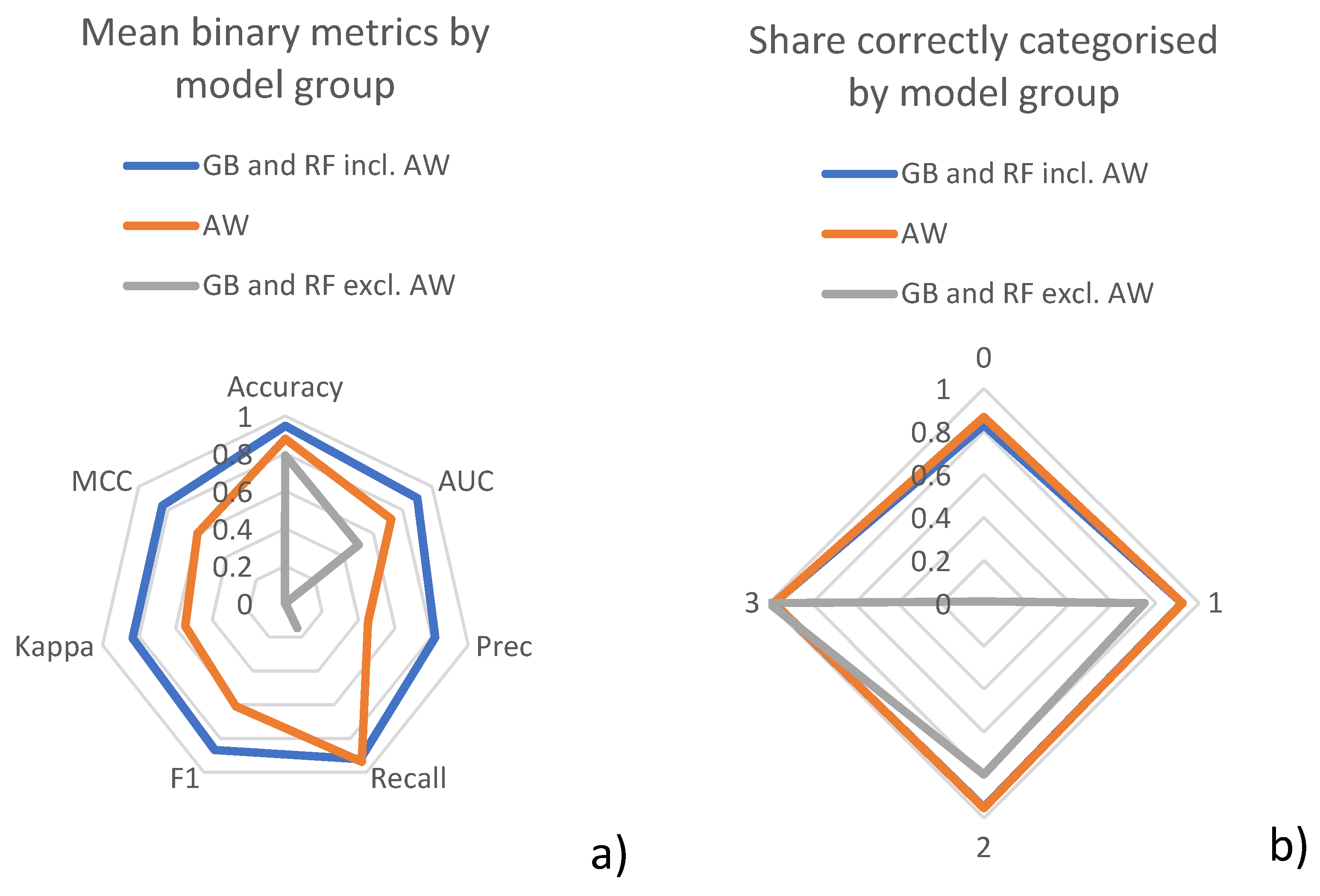
The key results are further summarised in Figure 2. The models have been grouped into three key groups. The first group, “GB and RF incl. AW”, shows the average result of all GB and RF that include the average weekly usage. “AW” is simply the result of the AW and “GB and RF excl. AW” is the result of the models unaware of average weekly usage.

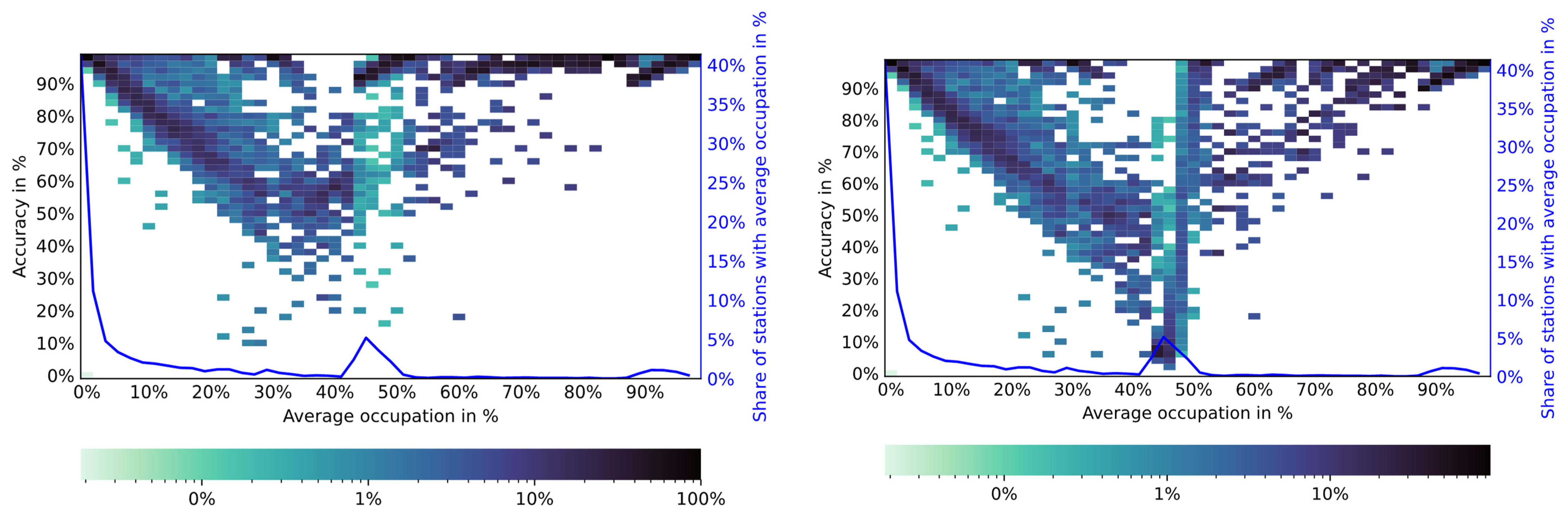
Another way to look at the results is presented in Figure 3, where the accuracy of GB with the 2021 dataset and all available data sources is compared to the accuracy for AW at the level of charging stations. It can be observed that all models are able to predict the usage of stations with either overall quite high or low usage. This is not surprising since a station that is nearly always/never used will likely be used/not be used in the future as well. The machine learning models, however, perform superiorly in the middle section, with stations being used between 30% and 50% of the time.

4.3. Feature Importance

When trying to use the prediction models in a real-world application, it is relevant to ensure that only those features are used that bring additional value to the prediction performance. While, theoretically, no damage should be done by including data with little additional value, the risk of overfitting and the effort required to warehouse and treat excess data sources both rise significantly with the amount of data used as features.

Table A1. Feature importance based on mean decrease in impurity of selected models, sorted by dataset first and then by MCC (i.e., same as in Table 4).

Model	Dataset	Include Average Week	Include Weather	Include Traffic	Feature Importance Based on Mean Decrease in Impurity
					Vacation	Long Weekend	Traffic	Traffic Relative	Weekday	Hour	Average Occupation	Temperature	Precipitation
GB	2021	TRUE	TRUE	TRUE	0.3%	0.0%	0.2%	0.0%	0.0%	0.1%	98.1%	1.3%	0.0%
GB	2021	TRUE	FALSE	TRUE	0.3%	0.0%	0.1%	0.0%	0.0%	0.0%	99.5%
RF	2021	TRUE	TRUE	TRUE	0.1%	0.0%	0.6%	0.1%	0.0%	0.1%	98.4%	0.8%	0.0%
RF	2021	TRUE	TRUE	FALSE	0.1%	0.0%			0.0%	0.1%	99.2%	0.7%	0.0%
GB	2021	TRUE	FALSE	FALSE	0.3%	0.0%			0.0%	0.0%	99.6%
RF	2021	TRUE	FALSE	FALSE	0.1%	0.0%			0.0%	0.0%	99.9%
RF	2021	TRUE	FALSE	TRUE	0.1%	0.0%	0.7%	0.1%	0.0%	0.0%	99.1%
GB	2021	TRUE	TRUE	FALSE	0.3%	0.0%			0.0%	0.1%	98.2%	1.3%	0.0%
GB	2021	FALSE	FALSE	TRUE	0.9%	0.3%	77.5%	19.1%	0.8%	1.5%
GB	2021	FALSE	TRUE	TRUE	1.0%	0.4%	75.5%	18.7%	0.7%	1.3%		2.4%	0.0%
RF	2021	FALSE	FALSE	FALSE	36.9%	4.9%			10.8%	47.5%
GB	2021	FALSE	FALSE	FALSE	37.1%	6.9%			13.2%	42.8%
RF	2021	FALSE	TRUE	TRUE	1.4%	0.2%	82.2%	11.1%	0.7%	1.9%		2.6%	0.1%
RF	2021	FALSE	FALSE	TRUE	1.4%	0.2%	83.0%	12.8%	0.7%	2.0%
GB	2021	FALSE	TRUE	FALSE	19.1%	12.5%			11.9%	26.5%		27.5%	2.4%
RF	2021	FALSE	TRUE	FALSE	19.0%	4.1%			10.7%	33.3%		30.7%	2.2%
GB	2019	TRUE	TRUE	FALSE	0.1%	0.0%			0.0%	0.2%	99.3%	0.3%	0.0%
GB	2019	TRUE	FALSE	FALSE	0.1%	0.0%			0.0%	0.1%	99.7%
RF	2019	TRUE	FALSE	FALSE	0.0%	0.0%			0.0%	0.1%	99.8%
RF	2019	TRUE	TRUE	FALSE	0.1%	0.0%			0.0%	0.2%	99.5%	0.2%	0.0%
GB	2019	FALSE	FALSE	FALSE	14.8%	14.5%			17.4%	53.3%
RF	2019	FALSE	FALSE	FALSE	14.2%	12.0%			16.0%	57.8%
RF	2019	FALSE	TRUE	FALSE	10.4%	4.9%			9.0%	30.6%		43.8%	1.2%
GB	2019	FALSE	TRUE	FALSE	13.1%	6.8%			10.6%	28.2%		39.8%	1.5%

shows the feature relevance using the mean decrease in impurity as a metric for the prediction models created in the context of this work. The AW is not included as it does not rely on external features.

5. Discussion

In this section, we discuss the results shown in the previous section. The structure is similar to the order in which the results were presented. We start with a short discussion of the model choice. The next three subsections discuss the usefulness of the different datasets and models given the prediction tasks. As a last content discussion, the feature importance is analysed. The section ends by discussing the limitations of the work done.

5.1. Model Choice

The comparison of a broad range of models was done to verify that the selected models in fact perform well in comparison to others. Since the project requires a measure of probability, the model choice was limited even before the comparison, but it is reassuring that GB and RF are among the better choices even in the more general task of binary classification. A Kappa and an MCC score of above 0.8 mean that the models have strong prediction quality in the binary challenge. Since the classification into the more diverse categories ranging from “very low” to “very high” is derived directly from the trained binary models’ probability, the same conclusion can be drawn about the choice of models for this application.

5.2. 2019 and 2021 Dataset

As can be seen in Table 4, the prediction performance in all major categories is significantly poorer for the longer dataset. The most likely explanation for this phenomenon is that Germany experienced dramatic changes in the time period that the models were unable to cover. One such change is the global COVID-19 pandemic, which resulted in three major lockdowns, resulting in significantly altered mobility patterns. With much more generous home office rules, the change in mobility patterns further had an effect outside the strict lockdowns. The second main change is the strong rise in EV sales. There were only 150,000 EVs on the road in the beginning of 2019 [45], but this number had risen to over 1 million by August 2021 [3]. Given that the mobility patterns and the number of users have dramatically changed over time, it is of little surprise that the models do not perform well when they have to predict the full time range.

The market is continuously changing, with increasing market shares of EVs [1], higher charging powers, and changing work modes, which may continue to change due to a broader acceptance of home-working [46]. This implies that there will be ongoing shifts in the use patterns of CSs. It therefore seems reasonable to assume that short training timeframes are more suitable for prediction than long ones.

5.3. Predicting Half-Occupancy

Looking at Table 4, three distinct groups can be observed. These are:

• GB and RF unaware of average weekly data
  All GB and RF models that are unaware of the average weekly data perform very poorly. Besides a seemingly reasonable accuracy of around 0.78, the MCC is 0 and AUC 0.5. The latter two indicate that the model has no predictive value. The reason for this is that the provided input features are an insufficient basis to predict a CS occupation of above 50% since the average occupation is too low and features are not unique enough.
• Average week model
  The average week model reaches a reasonable score in all major metrics. The relatively low recall, however, tells us that the model is unable to identify high CS occupation and earns most of its accuracy score by correctly predicting labels with low occupation rates. Given the goal of predicting usage spikes, this is clearly not ideal. This behaviour can be explained by the fact that only stations with an extremely high usage rate over the entire observed period during certain hours of the week would be correctly predicted as having a high occupation rate.
• GB and RF aware of average weekly data
  Once GB and RF are aware of the average weekly data, the prediction performance becomes much better. While there are small improvements in predictive quality if weather and traffic information is available, they do not make a strong contribution to station occupation. This occurs despite the fact that, individually, they show a strong correlation with station occupation. A reason for this could be that there are strong collinearities present. Traffic and station occupation, for instance, both show a similar pattern over the course of the day when using aggregated data. The results show that this effect holds true even when training detailed models.

The difference between the groups described in the second and third bullet points of the above list can also be observed in Figure 3. Unsurprisingly, both models achieve high accuracy for CSs with either a very high or a very low average occupation. Given that these CSs are either practically never used or always used, they are very likely to exhibit this behaviour in the test set as well. External features are irrelevant compared to the strong trend.

The difference is more pronounced in the middle segment, where CSs have more diverse usage. For these situations, GB (and RF, although not shown) have access to more information than AW and are thereby able to analyse the situation better. This allows these models to make much more accurate decisions in this segment, which is the reason that most binary metrics in Table 4 are much higher for GB and RF as compared to AW.

5.4. Predicting Categorised Values

Given that the ultimate goal of this work is to create a user-friendly way of displaying the likelihood that a CS is occupied, special attention is paid to the prediction of categorised values analysed through the confusion matrix. The 2021 data show a quite clear trend, where both RF and GB models are able to predict the exact category in over 80% of the predictions and predict the category itself or a nearby category at a rate of over 90%.

For users of the model, this high accuracy is good news. For most people, the difference between, for instance, “low” and “very low” is quite negligible, but the general tendency is of relevance. We can further see that GB and RF outperform AW significantly. This shows that simply taking the average weekly usage is insufficient when trying to make reasonably accurate predictions, but a correction using more models that are sophisticated is necessary.

As a third point, we can see, similar to the previous subsection, that the models unaware of the average weekly usage pattern are unable to make an accurate prediction. Virtually all predictions are in the categories “low” and “medium” since traffic, weather, and calendar data alone provide insufficient information for a prediction by itself. A consequence of this fact is that the suggested model can only be used in a real-world application if the stations have been operational for some time.

For the prediction of how a newly built station in a new location would likely be used, other tools are more adequate (see this paper’s literature review, as well as the literature review in [8,47]).

5.5. Feature Importance

As can be seen in Table A1, the average weekly occupation is by far the dominating factor if it is available. As was shown already earlier, both GB and RF only provide useful outputs once they gain access to the average weekly usage. It is consequently of little surprise that this feature is heavily used and reduces around 99% of impurity. The models, however, score significantly better than the AW in close to all settings. This seeming contradiction can be overcome by understanding that the average weekly usage essentially forms a starting point for the remainder of the decision trees. Upon visual inspection, most trees use the average occupation in the first two to three decision nodes, and only after this do they switch to other decision variables. The other features are consequently used to correct the average occupation for the specific circumstances that occur during a specific hour. This fact explains why the GB and RF have much higher prediction performance than the AW.

5.6. Limitations

In this work, several limitations must be considered. These are listed in the following.

• Market development
  The EV market has undergone tremendous changes in the studied period. The number of vehicles increased from approximately 150,000 vehicles in early 2019 to one million in 2021. Similar trends could be observed with respect to the number of CSs. At the same, vehicle range has increased significantly over time [9] and travel within Germany is now comfortably possible [48]. It seems probable that all these changes had an effect on infrastructure usage. Consequently, training and test data might in part be outdated, which the results in Table 4, including the 2019 dataset, also show.
• COVID-19 pandemic
  The COVID-19 pandemic has had an immense and lasting impact on mobility and travel patterns in Germany and worldwide. These developments are a second highly dynamic factor that the used models may not be able to reflect in detail.
• Availability of datasets
  One can think of various other aspects that probably increase prediction accuracy but for which we could not obtain datasets in this study. Examples of such data are events taking place (where visitors require recharging opportunities), hotel bookings (assuming that people need more public infrastructure if they are not at home), etc. If a reliable and quantifiable dataset can be obtained for these tasks, the prediction accuracy would likely increase further.

If the EV market and the COVID-19 pandemic should stabilise, it would certainly be of interest to study the topics in this paper again. We believe that it would, for instance, be critical to include seasonal patterns in future work, but could not do so here due to the fact that too much changed over a period of a single year. If researchers have access to datasets described in the last point of the Limitations list, a new study would certainly also be highly interesting and may create new insights into which features add value.

6. Conclusions

In this paper, we showed how the occupation level of a CS can be predicted accurately using data-driven methods. The models were able to achieve high scores in all standard metrics typically used in machine learning. We further showed how a binary training set might be used to create models that are then able to predict the more fine-grained categories of “very low” to “very high” occupation levels of public CI.

We further conclude that predicting future CS requires knowledge of past station usage. Since the usage patterns are currently changing quickly due to the COVID-19 pandemic and the rapidly growing market, it is sufficient to have knowledge of the near past. Longer datasets are not required. If this information is unavailable, at least the features available in this work were able to provide a useful prediction in the time resolution required. The addition of other datasets, such as traffic and weather data, increases model performance somewhat, but the impact is comparably small. Using a machine learning algorithm is sensible since the tested algorithms, GB and RF, scored significantly better than the simple average usage on a weekly basis.

References

- IEA. Global EV Outlook 2021; IEA: Paris, France. Available online: https://www.iea.org/reports/global-ev-outlook-2021 (accessed on 13 September 2021).
- Gorner, M.; Paoli, L. How Global Electric Car Sales Defied COVID-19 in 2020. Available online: https://www.iea.org/commentaries/how-global-electric-car-sales-defied-covid-19-in-2020 (accessed on 15 November 2021).
- Bundesregierung. Erstmals Rollen Eine Million Elektrofahrzeuge auf Deutschen Straßen: Mehr als 50 Prozent Dieser Elektrofahrzeuge Sind Rein Batteriebetrieben. Available online: https://www.bmwi.de/Redaktion/DE/Pressemitteilungen/2021/08/20210802-erstmals-rollen-eine-million-elektrofahrzeuge-auf-deutschen-strassen.html (accessed on 13 September 2021).
- Rogers, E.M. Diffusion of Innovations, 5th ed.; Riverside; Free Press: Amsterdam, The Netherlands, 2003; Available online: https://ebookcentral.proquest.com/lib/gbv/detail.action?docID=4935198 (accessed on 13 September 2021).
- Giansoldati, M.; Monte, A.; Scorrano, M. Barriers to the adoption of electric cars: Evidence from an Italian survey. Energy Policy 2020, 146, 111812. [Google Scholar] [CrossRef]
- She, Z.-Y.; Sun, Q.; Ma, J.-J.; Xie, B.-C. What are the barriers to widespread adoption of battery electric vehicles? A survey of public perception in Tianjin, China. Transp. Policy 2017, 56, 29–40. [Google Scholar] [CrossRef]
- ZLing, Z.; Cherry, C.R.; Wen, Y. Determining the Factors That Influence Electric Vehicle Adoption: A Stated Preference Survey Study in Beijing, China. Sustainability 2021, 13, 11719. [Google Scholar] [CrossRef]
- Hecht, C.; Das, S.; Bussar, C.; Sauer, D.U. Representative, empirical, real-world charging station usage characteristics and data in Germany. eTransportation 2020, 6, 100079. [Google Scholar] [CrossRef]
- Hecht, C.; Figgener, J.; Sauer, D.U. ISEAview—Elektromobilität; ISEA Insitute, RWTH Aachen: Aachen, Germany, 2021; Available online: https://www.doi.org/10.13140/RG.2.2.29327.51368 (accessed on 22 March 2021).
- Follmer, R.; Gruschwitz, D. Mobilität in Deutschland—MiD Kurzreport. Ausgabe 4.0; Studie von infas, DLR, IVT und infas 360 im Auftrag des Bundesministers für Verkehr und Digitale Infrastruktur: Bonn, Germany, 2019; Available online: http://www.mobilitaet-in-deutschland.de/pdf/infas_Mobilitaet_in_Deutschland_2017_Kurzreport.pdf (accessed on 22 June 2020).
- Figgener, J.; Tepe, B.; Rücker, F.; Schoeneberger, I.; Hecht, C.; Jossen, A.; Sauer, D.U. The Influence of Frequency Containment Reserve Flexibilization on the Economics of Electric Vehicle Fleet Operation. arXiv 2021, arXiv:2107.03489. [Google Scholar]
- Hecht, C. BeNutz LaSA: Bessere Nutzung von Ladeinfrastruktur durch Smarte Anreizsysteme. Available online: https://benutzlasa.de/ (accessed on 19 March 2021).
- Straka, M.; De Falco, P.; Ferruzzi, G.; Proto, D.; Van Der Poel, G.; Khormali, S.; Buzna, L. Predicting Popularity of Electric Vehicle Charging Infrastructure in Urban Context. IEEE Access 2020, 8, 11315–11327. [Google Scholar] [CrossRef]
- Viswanathan, S.; Appel, J.; Chang, L.; Man, I.V.; Saba, R.; Gamel, A. Development of an assessment model for predicting public electric vehicle charging stations. Eur. Transp. Res. Rev. 2018, 10, 1287. [Google Scholar] [CrossRef]
- Bi, R.; Xiao, J.; Viswanathan, V.; Knoll, A. Influence of Charging Behaviour Given Charging Station Placement at Existing Petrol Stations and Residential Car Park Locations in Singapore. Procedia Comput. Sci. 2016, 80, 335–344. [Google Scholar] [CrossRef] [Green Version]
- Ramachandran, A.; Balakrishna, A.; Kundzicz, P.; Neti, A. Predicting Electric Vehicle Charging Station Usage: Using Machine Learning to Estimate Individual Station Statistics from Physical Configurations of Charging Station Networks. arXiv 2018, arXiv:1804.00714. [Google Scholar]
- Bryden, T.S.; Hilton, G.; Cruden, A.; Holton, T. Electric vehicle fast charging station usage and power requirements. Energy 2018, 152, 322–332. [Google Scholar] [CrossRef]
- Majidpour, M. Time Series Prediction for Electric Vehicle Charging Load and Solar Power Generation in the Context of Smart Grid. Ph.D Thesis, University of California, Los Angeles, CA, USA, 2016. Available online: https://escholarship.org/uc/item/5gc4h0wh (accessed on 22 March 2021).
- Motz, M.; Huber, J.; Weinhardt, C. Forecasting BEV charging station occupancy at work places. INFORMATIK 2021, 2020, 771–781. [Google Scholar]
- Tian, Z.; Jung, T.; Wang, Y.; Zhang, F.; Tu, L.; Xu, C.; Tian, C.; Li, X.-Y. Real-Time Charging Station Recommendation System for Electric-Vehicle Taxis. IEEE Trans. Intell. Transp. Syst. 2016, 17, 3098–3109. [Google Scholar] [CrossRef]
- Panahi, D.; Deilami, S.; Masoum, M.A.S.; Islam, S. Forecasting plug-in electric vehicles load profile using artificial neural networks. In Proceedings of the 2015 Australasian Universities Power Engineering Conference (AUPEC), Wollongong, NSW, Australia, 27–30 September 2015; pp. 1–6. [Google Scholar]
- AlMaghrebi, A.; AlJuheshi, F.; Rafaie, M.; James, K.; Alahmad, M. Data-Driven Charging Demand Prediction at Public Charging Stations Using Supervised Machine Learning Regression Methods. Energies 2020, 13, 4231. [Google Scholar] [CrossRef]
- Frendo, O.; Graf, J.; Gaertner, N.; Stuckenschmidt, H. Data-driven smart charging for heterogeneous electric vehicle fleets. Energy AI 2020, 1, 100007. [Google Scholar] [CrossRef]
- Ullah, I.; Liu, K.; Yamamoto, T.; Zahid, M.; Jamal, A. Electric vehicle energy consumption prediction using stacked generalization: An ensemble learning approach. Int. J. Green Energy 2021, 18, 896–909. [Google Scholar] [CrossRef]
- Ullah, I.; Liu, K.; Yamamoto, T.; Al Mamlook, R.E.; Jamal, A. A comparative performance of machine learning algorithm to predict electric vehicles energy consumption: A path towards sustainability. Energy Environ. 2021. [Google Scholar] [CrossRef]
- Dias, G.M.; Bellalta, B.; Oechsner, S. Predicting occupancy trends in Barcelona’s bicycle service stations using open data. In Proceedings of the 2015 SAI Intelligent Systems Conference (IntelliSys), London, UK, 10–11 November 2015; pp. 439–445. [Google Scholar]
- Yoshida, A.; Yatsushiro, Y.; Hata, N.; Higurashi, T.; Tateiwa, N.; Wakamatsu, T.; Tanaka, A.; Nagamatsu, K.; Fujisawa, K. Practical End-to-End Repositioning Algorithm for Managing Bike-Sharing System. In Proceedings of the 2019 IEEE International Conference on Big Data (Big Data), Los Angeles, CA, USA, 9–12 December 2019; pp. 1251–1258. [Google Scholar]
- Sohrabi, S.; Paleti, R.; Balan, L.; Cetin, M. Real-time prediction of public bike sharing system demand using generalized extreme value count model. Transp. Res. Part A Policy Pract. 2020, 133, 325–336. [Google Scholar] [CrossRef]
- Almannaa, M.H.; Elhenawy, M.; Rakha, H.A. Dynamic linear models to predict bike availability in a bike sharing system. Int. J. Sustain. Transp. 2020, 14, 232–242. [Google Scholar] [CrossRef]
- Chen, B.; Pinelli, F.; Sinn, M.; Botea, A.; Calabrese, F. Uncertainty in urban mobility: Predicting waiting times for shared bicycles and parking lots. In Proceedings of the 16th International IEEE Conference on Intelligent Transportation Systems (ITSC 2013), The Hague, The Netherlands, 6–9 October 2013; pp. 53–58. [Google Scholar]
- Liu, D.; Dong, H.; Li, T.; Corcoran, J.; Ji, S. Vehicle scheduling approach and its practice to optimise public bicycle redistribution in Hangzhou. IET Intell. Transp. Syst. 2018, 12, 976–985. [Google Scholar] [CrossRef]
- Hua, M.; Chen, J.; Chen, X.; Gan, Z.; Wang, P.; Zhao, D. Forecasting usage and bike distribution of dockless bike-sharing using journey data. IET Intell. Transp. Syst. 2020, 14, 1647–1656. [Google Scholar] [CrossRef]
- Cagliero, L.; Cerquitelli, T.; Chiusano, S.; Garza, P.; Xiao, X. Predicting critical conditions in bicycle sharing systems. Computing 2017, 99, 39–57. [Google Scholar] [CrossRef]
- Lozano, A.; De Paz, J.F.; González, G.V.; De La Iglesia, D.H.; Bajo, J. Multi-Agent System for Demand Prediction and Trip Visualization in Bike Sharing Systems. Appl. Sci. 2018, 8, 67. [Google Scholar] [CrossRef] [Green Version]
- Yang, Z.; Hu, J.; Shu, Y.; Cheng, P.; Chen, J.; Moscibroda, T. Mobility Modeling and Prediction in Bike-Sharing Systems. In Proceedings of the 14th Annual International Conference on Mobile Systems, Applications, and Services, San Francisco, CA, USA, 14–18 June 2010; ACM Press: New York, NY, USA, 2016; Volume 06202016, pp. 165–178. [Google Scholar]
- OpenChargeAlliance. Open Charge Alliance—Global Platform for Open Protocols. Available online: https://www.openchargealliance.org/ (accessed on 19 March 2021).
- Ryanss and Dr-Prodigy. Holidays—PyPI. Available online: https://pypi.org/project/holidays (accessed on 19 March 2021).
- Freiling Digital GmbH. Kalenderdaten als ICS Datei Download—Ferienwiki. Available online: https://www.ferienwiki.de/exports/de (accessed on 19 March 2021).
- DWD Climate Data Center (CDC). Historical Hourly Station Observations of 2 m Air Temperature and Humidity for Germany, Version v006. Available online: https://opendata.dwd.de/climate_environment/CDC/observations_germany/climate/hourly/air_temperature/ (accessed on 7 May 2021).
- DWD Climate Data Center (CDC). Historical Hourly Station Observations of Precipitation for Germany, Version v006. Available online: https://opendata.dwd.de/climate_environment/CDC/observations_germany/climate/hourly/precipitation/ (accessed on 7 May 2021).
- ADAC Service GmbH. ADAC B2B. Available online: https://adac-b2b.com/ (accessed on 17 September 2021).
- Virtanen, P.; Gommers, R.; Oliphant, T.E.; Haberland, M.; Reddy, T.; Cournapeau, D.; Burovski, E.; Peterson, P.; Weckesser, W.; Bright, J.; et al. SciPy 1.0: Fundamental algorithms for scientific computing in Python. Nat. Methods 2020, 17, 261–272. [Google Scholar] [CrossRef] [PubMed] [Green Version]
- Ali, M. PyCaret: An Open Source, Low-Code Machine Learning Library in Python. Online: PyCaret. 2020. Available online: https://pycaret.org/ (accessed on 15 September 2021).
- Pedregosa, F.; Varoquaux, G.; Gramfort, A.; Michel, V.; Thirion, B.; Grisel, O.; Blondel, M.; Prettenhofer, P.; Weiss, R.; Dubourg, V.; et al. Scikit-learn: Machine Learning in Python. J. Mach. Learn. Res. 2011, 12, 2825–2830. [Google Scholar]
- Kraftfahrtbundesamt. FZ 1: Bestand an Kraftfahrzeugen und Kraftfahrzeuganhängern nach Zulassungsbezirken; Kraftfahrtbundesamt: Flensburg, Germany, 2020. [Google Scholar]
- Lund, S.; Madgavkar, A.; Manyika, J.; Smit, S.; Ellingrud, K.; Robinson, O. The future of work after COVID-19. McKinsey Global Institute. February 2021. Available online: https://www.mckinsey.com/featured-insights/future-of-work/the-future-of-work-after-covid-19 (accessed on 13 September 2021).
- Olk, C.; Trunschke, M.; Bussar, C.; Sauer, D.U. Empirical Study of Electric Vehicle Charging Infrastructure Usage in Ireland. In Proceedings of the 2019 4th IEEE Workshop on the Electronic Grid (eGRID), Xiamen, China, 11–14 November 2019; pp. 1–8. [Google Scholar]
- Hecht, C.; Victor, K.; Zurmühlen, S.; Sauer, D.U. Electric vehicle route planning using real-world charging infrastructure in Germany. eTransportation 2021, 10, 100143. [Google Scholar] [CrossRef]
Figure 1.
Boundaries for test predictions using the classification boundaries shown in Equations (4) and (5). The boundaries were chosen such that the group sizes are identical using GB and AW.
Figure 2.
Results of Table 4 grouped by model type and whether the average weekly data (AW) were used or not. Part (a) shows the results for binary metrics and (b) for the categorised results. Category “0” corresponds to the share of correctly assigned categories; “1” counts direct neighbour categories (e.g., “very low”–“medium” are still correct if “low” was the true value); “2” includes neighbours once removed; “3” neighbours twice removed.
Figure 3.
Accuracy of GB with all available inputs in 2021 (left) and of AW again for 2021 (right). The colour indicates which share of stations with the given average occupation was predicted with which accuracy. The heat map is constructed of rectangles with 2% edge length in both dimensions. Example of how to read: A dark green square corresponding to 80% with an average occupation of 50% and accuracy of 90% indicates that, for all stations with an average occupation of 50% to 52%, the prediction model achieved accuracy between 90% and 92% in 80% for all CS falling into the category. The blue line indicates what share of stations fell into each 2% block of average occupation.