
Digital Twin Concepts with Uncertainty for Nuclear Power Applications


1
Department of Nuclear Engineering and Radiological Sciences, University of Michigan, Ann Arbor, MI 48109, USA
2
Department of Mechanical Engineering, University of Michigan, Ann Arbor, MI 48109, USA
*
Author to whom correspondence should be addressed.
Energies 2021, 14(14), 4235; https://doi.org/10.3390/en14144235
Submission received: 20 May 2021
/
Revised: 30 June 2021
/
Accepted: 6 July 2021
/
Published: 14 July 2021
(This article belongs to the Special Issue Expanding Nuclear Applications and Technologies for a Clean Energy Future)
Abstract
:Digital Twins (DTs) are receiving considerable attention from multiple disciplines. Much of the literature at this time is dedicated to the conceptualization of digital twins, and associated enabling technologies and challenges. In this paper, we consider these propositions for the specific application of nuclear power. Our review finds that the current DT concepts are amenable to nuclear power systems, but benefit from some modifications and enhancements. Further, some areas of the existing modeling and simulation infrastructure around nuclear power systems are adaptable to DT development, while more recent efforts in advanced modeling and simulation are less suitable at this time. For nuclear power applications, DT development should rely first on mechanistic model-based methods to leverage the extensive experience and understanding of these systems. Model-free techniques can then be adopted to selectively, and correctively, augment limitations in the model-based approaches. Challenges to the realization of a DT are also discussed, with some being unique to nuclear engineering, however most are broader. A challenging aspect we discuss in detail for DTs is the incorporation of uncertainty quantification (UQ). Forward UQ enables the propagation of uncertainty from the digital representations to predict behavior of the physical asset. Similarly, inverse UQ allows for the incorporation of data from new measurements obtained from the physical asset back into the DT. Optimization under uncertainty facilitates decision support through the formal methods of optimal experimental design and design optimization that maximize information gain, or performance, of the physical asset in an uncertain environment.
1. Introduction
The concept of the digital twin (DT) is permeating across nearly all engineering disciplines, as well as other fields. The increased interest in DTs relates to their role in the Industry 4.0 revolution [1], and is driven by technology advances that bridge physical assets with digital models, e.g., the Internet of Things (IoT). Industries that do not successfully transition through this revolution will likely be diminished. In this regard, the nuclear power industry is no exception. The anticipated value of DTs in nuclear power can generally be taken as gains in efficiency and safety—both perpetual goals in nuclear power applications. The impact of such DTs could be far-reaching, including real-time monitoring that enables automation and predictive maintenance, accelerated development time, enhanced risk assessment, and optimization in various aspects of the system (e.g., operation, component design, fuel utilization, shielding, etc.). Therefore, DTs for nuclear power systems should be considered a key technology for expanding nuclear power applications. With the impetus of the world’s current climate crisis, carbon-free, clean energy technologies, like nuclear power, are critical to ensure the viability of our future.
According to the authors of [2,3], the DT terminology dates to the early 2000s, and it is usually credited to Grieves who later documented it in a white paper [4] from 2014. The U.S. Airforce in 2011 [5] and NASA in 2012 [6] defined the DT more completely for aerospace applications and identified it as a key technology. Several other definitions of DTs were also proposed prior to more contemporary efforts [7,8,9,10]. Many of the recent papers focus on generalizing the idea of the DT [2,3,11,12,13], as the earlier works were concerned specifically with aircraft, high-fidelity simulation, and structural mechanics.
Currently, there are many contemporary review articles on DTs focused on the definitions, challenges, enabling technologies, and opportunities [2,3,14,15]. (For readers interested in a comprehensive review of DTs, we recommend the work by Rasheed et al. [3], which has an extensive bibliography.). One recent review article on DTs identifies three distinct application areas: manufacturing, healthcare, and smarty city environments [2]. In this review, aircraft, power, and energy systems were all grouped under manufacturing. However, this review included only one paper each for power systems, aircraft, and energy systems. Therefore, the discussions in the aforementioned reviews tend to focus on these broader views with industrial processes generally lumped in with manufacturing, and ignore the specific considerations of any subdiscipline.
Works that are more specific to the nuclear engineering discipline include those in [16,17,18,19]. In [16,17], Garcia et al. mention DTs, but they do not review or advance DT concepts, nor provide clear or concise definitions of them. Rather, these works focus on the broader concepts of secure embedded intelligence and integrated state awareness, where DTs have a specific role. The DT concept is closely tied to Industry 4.0, and Lu et al. [18] provide a review of nuclear power plants in the context of AI and Industry 4.0. This work also mentions DTs, and advances the concept of a nuclear power plant as a Human-Cyber-Physical System, very much in the spirit of DTs, but limits the focus to AI-based approaches. Additionally, there is a review article in preparation by Lin et al. [19] that focuses on uncertainty quantification (UQ) of machine learning (ML) generated DTs for prognostics and diagnostics supporting autonomous management and control of nuclear power systems. The main contributions of this work are the review of ML methods to support DT creation and assessment, and how the software underlying the ML-based DTs may be evaluated in a risk-aware and regulatory setting. Overall, however, we make the observation that there is a notable dearth of literature on DTs for nuclear systems.
We do not seek to replicate the reviews for general DTs in this paper, nor do we seek to describe the technical details of a particular DT solution or software architecture. Instead, our aim is to convey the salient elements of some of these works and offer perspectives about the relationship to ongoing activities in the nuclear engineering community. With this paper we seek to add to the literature for DT concepts related to nuclear applications, and in keeping with the spirit of other contemporary works, we focus on understanding and defining the DT concept in the context of nuclear power. Specifically, the objective of this paper is to review and relate these broader works to the nuclear engineering community. We aim to accomplish this by identifying what aspects of DT development and enabling technologies are most appropriate for study and advancement by the nuclear engineering community, and where the community should be looking to adopt existing technologies. Much of the paper focuses on physics-based simulation technologies for DT development—rather than ML—and the importance of UQ in connecting the physical and digital assets. Further, we provide commentary on the recent directions and activities of research and development in nuclear power applications, and modeling and simulation (M&S). We also offer suggestions on how we might refocus some of current efforts to support DTs in nuclear power applications. In general, we will not focus on the aspects of risk-informed analysis or AI/ML methods as these are suitably covered by Lin et al. [19].
For the remainder of this paper, we first provide some background on nuclear power technology. Then, a review and discussion about the important details of defining DTs is given in Section 3 with a newly proposed definition for nuclear power applications. Section 4 reviews existing nuclear engineering M&S capabilities in the context of DTs. Next, in Section 5, we offer perspectives on the needs and challenges of developing and using DTs for nuclear power applications. This section focuses primarily on the computational and simulation aspects of DTs. Following this, in Section 6, we transition the discussion to UQ from a more technical angle. Here, we identify and examine challenges and promising methodologies for linking the physical and digital halves of the DT. Finally, we summarize the paper with some concluding remarks in Section 7 on the relevance of DTs as an enabling technology for nuclear power in a clean energy future.
2. Brief Overview of Nuclear Power Systems
Nuclear power systems produce heat energy through the fission process which is driven by the interaction of neutrons with the nucleus of an atom. In the fission process, heavy nuclides break apart and deposit their kinetic energy locally as heat. The primary element for fission in commercial energy production is uranium. The principle advantages of nuclear fission as a thermal energy source are its overall power density, long operation times without needing to refuel, and lack of carbon emissions.
In currently operating nuclear power systems, the heat produced by fission is transported away and typically used in a Rankine cycle to rotate a turbine to produce electricity. This is essentially the same power conversion cycle as combined-cycle natural gas plants and other fossil fueled power plants. Some example diagrams of existing reactor types are illustrated in Figure 1 to show some of the primary components in the system.
Advanced nuclear systems (also called Gen-IV reactors), which have yet to operate commercially (although there are a handful of historical examples), may use different power conversion cycles, such as a Brayton cycle or working fluids (such as molten salts). Simplified reactor system schematics of Generation IV reactor designs are given in Figure 2 to illustrate some of the main components in these nuclear power systems. To create a DT of a nuclear power system, these components—at least—would need to be digitized and modeled; however, in actual nuclear power systems, there can be thousands of components.
Because the power conversion systems for nuclear energy are similar to power conversion systems used in the fossil industry, there is considerable overlap in the components that are required for digitization to construct a digital twin. The defining aspect of nuclear power systems is the nuclear core. Although some other systems and components utilize highly specialized materials and are subject to unique degradation modes as a result of operating in intense radiation environments, the particular aspects of a nuclear power DT that differentiate it from other DT efforts derive from the presence of radiation and the physics resulting from the interaction of radiation with matter in the physical system. Consequently, much of our discussion throughout this manuscript focuses on these defining features.
For the modeling of nuclear power systems, the usual equations of structural mechanics and dynamics, fluid dynamics, and heat transfer are no different than other fields of engineering. In materials performance at the engineering scale, the physics are so complex that first principles equations are not as well defined, so empirical formulations, Arrhenius-like equations, and statistical mechanics are used to develop models that may be quite different from those found in other engineering disciplines. The equations that are most unique to the nuclear system are the Boltzmann neutron transport equation (NTE), Equation (1), and the nuclide transmutation and decay equation (often called the Bateman equation), Equation (2). There are also modified forms of the NTE that describe the transport of gamma rays, and charged particles, after introducing terms for electromagnetic forces. These equations are relevant to the transport of other particles in reactors, and are important to modeling the mechanisms for the detection of radiation.
In the time-dependent NTE shown by Equation (1), the fundamental unknown is the angular neutron flux, , which has dependent variables for its position in 3D space, ; its direction of flight, (described by two independent angles); its energy, E (or velocity, v); and time, t. Physically it represents the number of neutron tracks generated per unit volume for a given speed and direction at a moment in time. The NTE is a conservation equation for the time rate of change of the angular flux where neutrons are lost by leaking out of the system or colliding with a nucleus. Neutrons of different energies and directions of flight may scatter into a particular unit of phase space, be generated through fission, or some other external source, Q. The probability that a neutron collides with a nucleus is described by the total macroscopic cross section, , where some of those interactions may result in a scattering event or a fission event. The corresponding probability for scattering from another direction, , and energy, , into E and is described by the scattering kernel, . The probability that a neutron–nucleus interaction results in a fission is given by the macroscopic fission cross section, . On average, a fission event produces neutrons with the probability of the neutrons being emitted at E given by . The remaining fraction of neutrons emitted, , are delayed. These neutrons are emitted through the radioactive decay of precursors, , at a rate of , and have a different emission spectrum, , than the prompt neutrons. The precursor concentrations have their own set of differential equations that follow as simplifications to Equation (2), and we give these in Equation (5). Reactors operate by sustaining a chain reaction, so during normal operation, the derivative of the angular flux with respect to time is essentially zero.
The Bateman equation describes the evolution of the materials in the reactor subject to neutron bombardment and radioactive decay. It is also a conservation equation. The time constants in this equation can vary from microseconds to millions of years. For practical engineering applications, important effects described by Equation (2) occur on time scales from days to months. The solution of this equation is essential to knowing the state of the materials in the reactor, its resulting criticality (whether or not it can sustain a chain reaction), and how much fuel is left. In this equation, represents the number density of isotope i. The system of differential equations can include up to every known isotope in the chart of nuclides, which is more than 2000. is the decay constant for radioactive decay of the nuclide; is the fraction of decays of nuclide j resulting in formation of nuclide i; is the microscopic absorption cross section; is the fraction of neutron absorptions in nuclide j resulting in the formation of nuclide i; and is the scalar neutron flux, which is the angular flux integrated over . For non-solid fuels, the Bateman equation must be modified to include an advection term to account for the motion of nuclides in space.
Common approximations of the NTE include the neutron diffusion equation, Equation (3), which neglects the dependence on the direction of flight for neutrons and assumes that they are distributed isotropically in angle, and the point kinetics equations, Equation (4), that ignores the spatial and energy dependence of the neutrons in a reactor. Although simpler, these equations are still widely used in reactor analysis, and in a broader sense may be understood as reduced order models of Equation (1).
In the diffusion equation, most of the terms have the same meaning as given in Equation (1), and is the scalar neutron flux. The main approximation introduced in the diffusion equation is that the leakage (advection) operator is replaced by a diffusion operator with a diffusion coefficient, . Essentially this assumes that how neutrons move through a system can be sufficiently described by Fick’s Law of Diffusion.
The point kinetics equations describe the time dependence of the power, P of a point-reactor, where is the reactivity that results from perturbations to the system by passive feedback or operator intervention, and is the prompt neutron lifetime. We also introduce the other set of important differential equations for the production of delayed neutrons that are emitted milliseconds to 10 s of seconds after a fission event (rather than simultaneously with the fission event). The delayed neutron precursors, , correspond to daughter nuclides produced from fission; however, typically these data are obtained from regression models such that there are 6 or 8 delayed neutron precursors instead of the actual dozens of nuclides emitting neutrons. is the fraction of delayed neutrons emitted per fission by precursor group k, where is the total delayed neutron fraction.
In summary, these are some examples of the types of nuclear power systems for which we seek a digital twin. Further, the first-principles equations unique to nuclear power systems, and common approximations to them used in regular engineering analysis, were presented and discussed to provide context to the underlying problems that must be simulated that are unique to a nuclear power system DT.
3. Defining Digital Twins for Nuclear Power Systems
The concept of twins are not new in nuclear power. Since the beginning of the commercial nuclear power industry, it has been practically standard practice to commission a duplicate control room for training purposes. In some of the early U.S. Government research programs for developing reactor systems, physical twin assets were also used. Since that time however, there has not been much innovation or advancement in the concepts of twinning. To be sure there have been significant advances in the technology underlying the various components, their design, and associated means of making measurements, but there has not been much in the way of conceiving of the physical systems and their twins or their use in a way that is fundamentally different. This is contrasted with the recent interests around the notion of the DT, particularly the high-fidelity kind, which is essentially made possible by the incredible advances in computers and simulation. M&S has now matured to a point that researchers in this area think it is possible, and imminent, to be able to create a DT. Exactly how that may be done is the focus of the Section 5. Prior to that, consistent, pedantic definitions of the DT for nuclear applications are needed.
3.1. Review of Digital Twin Definitions
Presently, the definition of a DT is quite broad and varies. This is due to the wide range of disciplines interested in DTs. Several definitions for DTs often contain nuanced but significant differences. What we are interested in elucidating in this section are the key characteristics that lead to these subtle differences and how to best organize this information into a conceptual model amenable to understanding the application of DTs to nuclear reactor systems.
Like the work by Fuller et al. [2], we start with a short review of some of the definitions given previously:
- Tuegel et al. [5] define the DT as being “ultrarealistic in geometric detail, including manufacturing anomalies, and in material detail, including the statistical microstructure level, specific to this aircraft tail number”. Here, the DT concept is focused on high-fidelity simulation by the finite element method (FEM) and computational fluid dynamics (CFD) for the prediction and management of the structural life of aircraft. The authors note that another key feature of their concept is the ability to “translate uncertainties in inputs into probabilities of obtaining various structural outcomes”.
- Glaessgen and Stargel [6] have a similar definition centering on ultra-high-fidelity simulation being integrated with a vehicle’s health management system. In this paper, the authors focus more on certification of the vehicles and a reliance on the assumed similitude of data used for certification. They identify this as a shortcoming to be addressed by DTs. Their definition for a DT is “an integrated multiphysics, multiscale, probabilistic simulation of an as-built vehicle or system that uses the best available physical models, sensor updates, fleet history, etc., to mirror the life of its corresponding flying twin”.
- Boschert and Rosen [7] provide a very general definition with “the Digital Twin itself refers to a comprehensive physical and functional description of a component, product or system, which includes more or less all information which could be useful in all—the current and subsequent—life cycle phases”. Here, the authors acknowledge that the DT concept is variable in terms of where it is applied in the product life cycle and the overall fidelity of data and models encompassed.
- Chen [8] similarly broadens the usage of DT and defines it as “a computerized model of a physical device or system that represents all functional features and links with the working elements”.
- Schluse et al. [10] take a slightly different perspective on DTs focusing on the value as an asset for experimentation. Nevertheless, many of the same fundamental requirements arise from their definition of experimental DTs as “a one-to-one replica of a real system incorporating all components and aspects relevant to use simulations for engineering purposes but also inside the real system during real-world operations”.
- Tao et al. [21] describe the DT in a few ways. First, it is a concept “associated with cyber-physical integration.“ Further, DTs create “high-fidelity virtual models of physical objects in virtual space in order to simulate their behaviors in the real world and provide feedback”, and “reflects a bi-directional dynamic mapping process”.
- Rasheed et al. [3] state that a “Digital twin can be defined as a virtual representation of a physical asset enabled through data and simulators for real-time prediction, optimization, monitoring, controlling, and improved decision making”.
- Lin et al. [19] also offer a good definition with: “A DT is a digital representation of a physical asset or system that relies on real-time and history data for inferring complete reactor states, finding available control actions, predicting future transients, and identifying the most preferred actions”.
3.2. Analysis of Key Characteristics
From the selected definitions given above, a few commonalities stand out: high-fidelity simulations, integration of calculated and measured quantities, detailed equivalence with a unique physical system, and application over a product’s/asset’s life cycle. Some definitions differ on the degree of equivalence between the digital and physical twins, noting that every detail is important or there may be only a subset of information that is relevant. Some definitions denote real-time simulation capability; others acknowledge the need for probabilistic methods. Several of the definitions describe the DT in the context of its application (e.g., prediction and management of the structural life or optimal control), although this application may vary.
3.3. Proposed Definition
In proposing our definition of the DT and related concepts, we draw from the concepts described by Fuller et al. [2]. However, we find these definitions by themselves lacking the context of a life cycle, so our definition expands these to exist within the life cycle laid out by Boschert et al. [7].
Fuller et al. [2] develop a taxonomy of three definitions that differentiate concepts based on information flow between the physical and digital assets, and categorize two of these as misconceptions. Their taxonomy defines digital models, digital shadows, and digital twins. We consider each of these valid, rather than some being misconceptions, as they each serve a distinct function in the life cycle to be described later. This differs from definition put forth by Lin et al. [19] where a DT is defined in terms of its function (intended use), its model (how it is developed), and interface (how information is communicated to the operator).
We propose the use of Fuller’s taxonomy as these definitions are relational with clear features, and do not necessarily preclude aspects of Lin’s conceptualization. The conceptual relation of the digital model, digital shadow, and digital twin is illustrated by Figure 3. As an example, in this figure, photographs of the Ford Nuclear Reactor represent the physical asset. Below this are a collection of images comprising digital representations of the Ford Nuclear Reactor. The digital representations include component models, simulation results, and virtual environments. The blue ovals represent the digital objects that comprise the digital model, digital shadow, and digital twin; the arrows illustrate the relationships and information exchange among these digital objects.
Our interpretation of Fuller’s Taxonomy is as follows:
- The digital model may or may not be associated with a physical asset. Thus, it need not integrate with physically measured or sensed quantities. This is how we might think of most of the existing M&S efforts in nuclear engineering. Full simulation models of planned or existing reactors, and their systems and components, capable of simulating the system physics and dynamics comprise the digital model. What distinguishes the digital model from the digital twin is that information generated by the digital model is not automatically integrated with the physical asset.
- The digital shadow extends the digital model by incorporating information from an existing physical asset to update the digital model, but does not utilize any information generated by the digital representation in the physical asset. We note that digital representations of historic facilities that no longer exist can qualify as digital shadows. The inverse of the digital shadow, where information only flows from a digital model to a physical asset, is not a coherent paradigm for useful engineering analysis as there is a physical system operating with essentially no connection to reality. Therefore, this situation is not explicitly defined or discussed further (For the curious reader, this paradigm essentially aligns with Plato’s Allegory of the Cave [22] or Putnam’s more contemporary “Brain in a vat” [23]).
- The digital twin is therefore the “closed loop” model of the physical asset and the digital representation(s). The digital twin exchanges information in real-time with the physical system to update its state and perform predictive calculations that are then used to inform decisions and control actions on the physical asset.
The definitions above do not necessarily clarify use or differentiate meaning within the context of a life cycle. Thus, we expand these definitions to describe how they should be used in the various phases of the physical asset’s life cycle. For the life cycle phases, we adapt those definitions from Boschert et al. [7]. The sequence of phases are shown in Figure 4 and include
- the initial conceptual design,
- the engineering design,
- procurement and construction,
- the operational phase that undergoes intermediate service, and
- and finally the decommissioning phase.
The lifetimes of the various digital objects are illustrated below with the life cycle phases in Figure 4. This figure shows that the digital model is the initial point of creation and may persist indefinitely. The lifetime of the digital twin is fully coincident with the lifetime of the physical asset. If there is no asset, there is no digital twin. Beyond the lifetime of the twin there is the digital shadow. The shadow can also exist coincidentally with the physical asset. Moreover, the shadow can exist indefinitely as integration of data from the physical asset may be manual. This recognizes the value of destructive testing and post-irradiation examinations of various components of the plant, where there can still be valuable information learned, and integrated into the digital object to refine the underlying models for the next generation of products.
The last aspect of our proposed definition is not to presume a single model, instance, fidelity, or physics in the digital representation. Rather, the digital object may be able to provide multiple models at the appropriate fidelity. This detail was not a part of the initial definitions of digital twins [5], but as these definitions evolved, it was incorporated [7]. The desire to have varying fidelity is one of the unique challenges that we discuss further in Section 5.
To summarize, the definition we propose for the DT includes the following components:
- Prior to the existence of any information exchange between the digital and physical assets, the digital object is described as a digital model. This often encompasses the conceptual and engineering design phases.
- The digital model may exist alongside the physical twin and indefinitely, if there is no information exchange with the physical asset.
- Following the creation of a physical asset, a digital shadow may be created that incorporates information from the physical asset in either an automated or manual sense, but it does not provide information back to the physical asset.
- The digital shadow may also persist indefinitely.
- The digital twin exists only as long as there is a physical asset.
- The digital twin has real-time, automated, two-way information exchange between the digital representation and physical asset.
- The digital twin may involve a set of models of varying fidelity and complexity.
- A digital twin has a corresponding digital model and digital shadow. The digital model and digital shadow are specific aspects of the twin.
In the remainder of this paper, we refer to the collection of these digital objects simply as the digital twin.
DTs should include a physical and functional description of all systems, structures, and components that captures as much detail as possible that is useful for any analysis, real-time prediction, monitoring, or control in any phase of the life cycle. The requirements and enabling technologies for the digital representations are discussed in Section 5. Next, we consider historical and contemporary digital representations of nuclear power systems to compare their capabilities to our definition of the digital twin.
4. Historical and Contemporary Digital Representations of Nuclear Power Systems
Several simulation capabilities for nuclear systems have been developed over the past 60 years. Advancing M&S capabilities of nuclear power systems has also been a key area of research in the past decade. Furthermore, there are numerous commercial tools not specific to nuclear power systems that have features to support DTs.
4.1. Common Nuclear Engineering Simulation Tools
The first tool we focus on is the plant simulator. Plant simulators have been around for several decades. They are generally full-scope and real-time—two attributes often desired of DTs. Their use is historically for training, and oftentimes includes a (physical or digital) duplicate of the control room. These replica control rooms are even known to be kept up to date with the minutiae of the real control room with details such as scratched surfaces or replaced instruments. Two commercial vendors for plant simulators are Western Services Corporation with their 3KEYMASTER platform that relies on RELAP5-3D [24] for system thermal-hydraulics, MARS [25] for core thermal hydraulics, and NESTLE [26] for core neutronics among other components. The other commercial vendor is GSE Solutions, which has their Generic PWR product (GPWR), but is also developing new build simulators for NuScale, AP1000, mPower, and the PBMR. We mention these as important technologies because they are full-scope, and they are real-time. They are not necessarily high-fidelity, and it is not clear how they might be adapted to integrate real-time information from a physical asset, or provide predictive capabilities. Nevertheless, they have clearly defined the necessary computational resource and modeling requirements to support the full-scope, real-time simulation of a plant. These contemporary products essentially run on single-core desktops with 2–3 GHz processors at real-time, or faster than real-time. This is in stark contrast to the high-fidelity tools to be discussed momentarily.
To accomplish this in the GPWR, the SimExec engine manages the dynamic execution of the various models for each component at the associated time intervals and maintains a master state of a few thousand state variables. To run real-time, component models are essentially lumped parameter dynamics models with strict execution time requirements (e.g., the model for component x must execute at 7 Hz). This engine can also integrate with a highly realistic interactive digitization of an actual control room if needed.
The requirements for plant simulators were detailed some time ago by Wiltshire in 1986 [27]. In that paper, Wiltshire describes a state-of-the-art system with the simulation requirements for an advanced gas reactor simulator. For a full-scope system, there are not only differential equations, but also algebraic (arising from property correlations and definitions of coefficients) and boolean systems of equations (arising from diagnostics). Table 1 summarizes the orders of magnitude in unknowns for some various components based on the information in [27] and more recent estimates. We note that Wiltshire describes a hardware system that uses 52 parallel computers, while today much of this is calculated on a single processor.
Beyond the full-scope plant simulator, the nuclear engineering community has focused considerable efforts on the system dynamics models with codes such as TRACE [28] and RELAP, which we note are already a part of these simulators in some cases. However, it is likely the versions in the simulator are not the most advanced form of these tools or necessarily use the highest fidelity representation of the plant. In addition to the system dynamics, the core modeling is the other area that receives considerable attention in terms of the tool development because the physics involved in the reactor are specific to the nuclear engineering discipline. The industry standard tool here is SIMULATE [29], which solves for the core power distribution and dynamic response—at least for light water reactors. For advanced reactors, DIF3D [30] is still the standard for non-pebble bed designs. In pebble bed designs, the core modeling tools are VSOP [31] and AGREE [32]. Reactor vendor specific tools also exist.
The high-fidelity simulation tools for plants thus far have mainly focused on individual components. The recent programs supporting development of these next generation tools were CASL [33], and now NEAMS [34]. Many of the tools developed under NEAMS are finite element-based, while under CASL, the VERA software [35] was an amalgam of models and codes, with the most novel contribution being the core simulator, VERA-CS [36]. The NEAMS finite element tools are generally based on the MOOSE framework [37]. From the MOOSE framework, there is also a suite (or zoo) of applications implementing various physics for modeling various components. For advanced reactor systems analysis, the SAM [38] code is also in development based on the MOOSE framework.
The tools described thus far are all mechanistic in nature—they arise from physically based governing partial differential equations. Beyond these mechanistic tools, the RAVEN framework [39] provides capabilities to support users with reduced order model (ROM) construction, statistical analysis, UQ, probabilistic risk assessment, and others. In a sense, RAVEN is designed to integrate with the mechanistic tools to exercise its capabilities.
Collectively, these tools do not rise to the level of supporting a DT on their own. They do, however, meet the criteria for a digital model, but this should not be surprising. In the nuclear engineering community, the last decade of research focus has been primarily on advancing the M&S capabilities that support digital models. As a result, we have several new codes and a program for advancing the fidelity of the mechanistic models through the adoption of more computationally expensive models. Nearly all of the NEAMS tools are designed to run in parallel on high-performance computing (HPC) systems, and are far from being able to provide value for real-time DTs. However, they can still serve a role in support of DTs as a basis for ROM construction, and other ways we will discuss in Section 5.1.3. Beyond this role however, the investments in high-fidelity simulation may not yield much return in the DT space without further advances.
4.2. Relevant Non-Nuclear Commercial Simulation Tools
Outside of nuclear engineering, there has been considerable progress in providing capabilities to support DTs. From the modeling side, any commercial software suite for dynamic systems modeling is capable of developing a full-scope, real-time digital model like the nuclear plant simulator. Some of these commercial tools at present are: Simulink, SimulationX, Dymola, MapleSim, 20sim, ANSYS Twin Builder, MSC Apex, etc. These products are generally far ahead of the corresponding U.S. Department of Energy (DOE) counterparts in terms of their overall feature set and capabilities for usability. However, beyond the physics for thermal-fluids and structural mechanics modeling, nearly all of them do not contain representations of the requisite physics for nuclear power applications described in Section 2.
This observation presents a conundrum about where to put forth effort. Should the M&S community work to integrate their capabilities with commercial tools or should they expend the effort to bring the quality and capabilities of their existing tools to the level of the commercial tools? This is a complicated question that the authors will forgo proposing an answer to. However, in the next section we discuss some tangible opportunities that relate to this consideration.
4.3. Emerging Tools and Capabilities
The emerging capabilities for DTs in the nuclear arena have both digital and physical components. On the digital side, there has been a notable investment in Modelica-based [40] models through the TRANSFORM library [41] and by the Integrated Energy Systems group at the Idaho National Laboratory (INL) where they have recently built system dynamics models of the NuScale reactor [42]. These models are notable for demonstrating the capabilities to model the dynamics of nuclear systems using Modelica, which is a modeling language that is arguably the most appropriate for DT applications. The emerging physical assets that present good opportunities are those under development in the microreactor program, and in particular the MAGNET [43] test bed. The Compact Integral Effects Test (CIET) facility has also been modeled with TRANSFORM [44] and SAM [45]. There is also an effort that has just started for developing and demonstrating a DT in the SAFARI project [46]; which is one of many recent ARPA-E funded projects under the GEMINA program with a DT component [47,48,49,50]. Last, the recently demonstrated KRUSTY experiments in the Kilopower project [51] demonstrated good prediction from the digital models and measured high quality data.
Thus, these recent and emerging tools and facilities represent an existing foundation on which one can build towards a functional DT. However, there is not yet an automated connection between the physically measured quantities and the digital models. Consequently, additional work is needed to realize nuclear system DTs. This is what we discuss next.
5. Enabling Technologies and Challenges for Digital Twins of Nuclear Power Systems
In this section, we describe the enabling technologies to realize nuclear DTs adhering to the definitions developed in Section 3. We focus on where contributions should be made by the nuclear engineering community. Moreover, technologies that are sufficiently mature, although not sufficiently familiar to the nuclear engineering community, where contributions are not necessarily needed, are also identified. Finally, some potential approaches to realizing a nuclear DT and their challenges are described. Since a significant aspect to the challenges and enabling technologies is in the area of UQ, Section 6 is devoted entirely to this topic.
5.1. Enabling Technologies
5.1.1. System Dynamics Modeling
System dynamics models are well established in several engineering disciplines. The evidence for this is in the plethora of multidisciplinary commercial simulation tools listed in Section 4.2. There is also an extensive history of their application in nuclear power systems. This is an enabling technology for DTs that will likely not require any revolutionary developments or contributions. Codes like TRACE, RELAP, and SAM are all systems dynamics codes developed specifically for nuclear reactor applications. We can think of these models as lumped parameter systems of varying fidelity—although the aforementioned examples are capable of capturing considerably more complex physics. Lumped parameter models can be sufficiently accurate and sufficiently inexpensive to evaluate. This has been proven repeatedly, as demonstrated by the examples of the simulators described in Section 4.1. Where system dynamics models typically fall short is in the applicability of their coefficients. In these models, the ROMs are known and can be rigorously derived with some assumptions (e.g., the point kinetics equations). The physics and applicability of these models rely almost entirely on the coefficients. The coefficients are the physics. Therefore, the challenge with system dynamics models is in having a way to adapt or recalibrate the coefficients to better match a physical asset’s behavior.
5.1.2. Model Based Controllers
One promising role for DTs in nuclear engineering is that they will support autonomous control and operation. Numerous methods exist in controls engineering, and we suggest that model-based controllers are the specific enabling technology for DTs. Model-based control systems rely on some underlying model that is reasonably predictive of the system dynamics. Several examples of model based control exist for nuclear power systems [52,53,54,55], and are generally applied to the core power, but may be used for other components or quantities of interest [56,57]. These models are typically lightweight so as to meet requirements for real-time execution and may be constructed rigorously through physics-based methods, statistical methods, purely data-driven approaches, or ML. Model predictive control (MPC) [58] is one example of model-based control with several variants that extend the underlying method to be robust in the presence of noise [59], applicable to nonlinear systems [60], or incorporate some ML methods [61]. We propose that model-based control is superior to model-free controllers (e.g., PID) because it is easier to make guarantees about the limits of the controller’s behavior and explainability is more easily achieved. Furthermore, in most cases we have a good sense of what the mechanistic model is, and purely model-free methods ignore this knowledge.
5.1.3. Automated ROM Construction
Another key technology for DT development will be automated ROM construction. There is more than 60 years of digital models of nuclear systems and many of these are not real-time. The simulation components of the DT will need to be primarily real-time. In any situation where an existing digital model is not real-time, it is amenable to representation as a ROM. As the digital models span a range of codes, models, tools, inputs, etc., having an automated way to produce a ROM will be a key enabling technology to seamlessly generate the necessary pieces to build a DT. There are numerous techniques that exist to produce ROMs. Some of these are given in Figure 5, illustrating how they might relate to other models, and one another, in terms of their knowledge of the physics and complexity. Any of these approaches, and others, are suitable for ROM construction. Although we suggest that knowledge of the physics being modeled by the ROM should be used to prioritize what technique is used.
Some capabilities exist in this regard through RAVEN [39], and they have been successfully demonstrated for risk-informed safety margin characterization [62]. However, the full spectrum of model order reduction methods is not available, so some contributions could be made here. An additional, practical, and critical consideration for automated ROM construction tools is ease of use by the community. To have tangible gains in productivity, modelers should expect to put forth as little effort as possible to create a ROM. Therefore, usability and flexibility should be the focus of this effort, not necessarily novel contributions to model order reduction techniques. Opportunities for novel contributions still exist though, but these should focus on developing a priori and a posterior error estimates of the ROM construction techniques to facilitate confidence in the usability and flexibility.
5.1.4. Functional Mockup Interfaces
The functional mockup interface (FMI) [63] is an open standard for a software interface to facilitate model exchange and co-simulation. This is an enabling technology because of the need to integrate different models of different fidelities involving different physics. Effectively, FMI standardizes an interface for coupling computational models independent of the tools. It uses a combination of XML files for describing the model contents and interface, and C-interfaces, shared libraries, or source code to provide a means to execute the code. There have been numerous attempts in the nuclear engineering community to develop such a capability [64,65,66,67,68]. However, none of these have seen broad adoption because they are largely tool- or framework-based. Our recommendation is that this standard be adopted to facilitate interaction with commercial tools and various software tools developed within the nuclear engineering community. Furthermore, the standard can support integration with physically sensed data and extended reality (either augmented or virtual). Presently, the standard is supported by several international experts and industry entities. We present Figure 6 from Touran et al. [68] as an example of the various interfaces that can exist for a nuclear energy DT; here, each of the interfaces could be implemented with FMI enabling broad interoperability with other commercial or open source tools.
5.2. A Digital Twin Paradigm
As we noted earlier, much of the necessary theory for the enabling technologies of DTs, and in some cases the technology itself, exists in some form. Therefore, we offer the opinion that the development and realization of a DT is primarily an applied research area, as opposed to a basic research activity. Our paradigm for the DT–physical asset interaction is illustrated in Figure 7. In this figure, the DT is a real-time dynamics model based on mechanistic models. This model calculates predicted responses and control actions for the DT, and receives inputs from the physical asset. It is assumed to contain various levels of controllers and decision making frameworks. This is to execute all in real-time and uses FMI as the basis of information exchange (or similar standard). Below the FMI-based communication layer is an offline—but on-demand—capability that uses resources that are slower than real-time. This also includes some data repository component for recording the history of the DT operation. Use of this on-demand resource would be managed by Optimal Experimental Design methods described in Section 6.3. The on-demand capabilities would likely consist of data-driven approaches to make sense of the sensed data and the existing high-fidelity M&S capabilities in nuclear reactor analysis.
The purpose of the on-demand capabilities is to evaluate the inconsistencies in the simplified real-time dynamics of the DT and, through ML processes (whether they are statistics-based, involve regression, or use neural networks), provide corrections to the DT. These corrections may account for changes in model coefficients due to the natural evolution of the physical asset (e.g., burnup, lower power states, high power states, etc.) or known limitations of the model (e.g., due to assumptions like linearity). We see this as one way to make use of the existing advanced M&S capabilities in NEAMS.
To achieve this paradigm using the aforementioned technologies there are several challenges that we now describe.
5.3. Challenges to Realizing Digital Twins
5.3.1. Security
As nuclear power systems represent sensitive and critical infrastructure, security of the information around the DTs should be considered a necessary requirement. Information security for DTs though should not be something developed by nuclear engineers, instead the community should consider itself a user of this technology. As a challenge, what is needed in this area is the proper engagement of experts in the field of cyber-physical system security to ensure the requirements of nuclear power applications are captured. Trying to devise our own solutions to the security problem are likely misguided. As an example, standards for IoT systems security are already in development [69]. Further, the notion of secure embedded intelligence [16] could be leveraged to devise solutions to this challenge.
5.3.2. Integration with Prognostics and Health Management
A recognized area for value extraction from DTs is in prognostics and health management (PHM). PHM appears repeatedly across multiple potential DT applications. The exact manner in which PHM-related data integrates with DTs remains unclear, specifically how the data is used as it is collected from the physical asset. Some proof-of-concepts for integration with PHM have been demonstrated [70] through using the enabling technologies mentioned in Section 5. A similar approach could be leveraged for nuclear power applications; however, this area represents one of the key challenges where the nuclear engineering community will need to engage the broader PHM community to develop novel solutions.
5.3.3. Data Collection, Curation, Transmission, and Integration
The tasks of data collection from sensors, curation of this data, and transmission and integration of the sensor data into the DT will likely present substantial challenges. However, all of these challenges are expected to be practical in nature, which is not to dismiss their importance. A DT must be able to perform these tasks. There is nothing theoretically complex about them, but they should be expected to be tedious, error-prone, and initially unreliable. For nuclear power system DTs, these capabilities should ideally be “turn-key”. Furthermore, these capabilities more generally fall under the capabilities of IoT infrastructure–where there are notable advancements happening rapidly. For example, the problem of localization of either people or radiological material inside a nuclear facility is paramount, but devising solutions to this problem like Pascale et al. [71] is not necessarily within the domain of expertise of nuclear engineers. Consequently, our suggestion is that these issues be addressed by IoT experts. A possible exception to this would be for nuclear engineers to engage with IoT experts to ensure the reliability of IoT in harsh environments (e.g., high temperature and high radiation).
5.3.4. Integration with Risk Assessments
DTs must be integrated with risk assessments for regulatory acceptance. Moreover, integration with risk will likely be necessary to achieve the benefits from increased reliability of the physical system and improved automation. One way that the integration of the DT and risk has been envisioned is through dynamic probabilistic risk assessment. Traditional Probabilistic Risk Assessment (PRA)—which is not dynamic—is one of the cornerstone safety analysis methodologies for reactor licensing. Through traditional PRA, fault-trees and event-trees are developed with appropriate probabilities of failures and events, then analyzed to produce core damage frequencies. The core damage frequency is defined as the probability of core damage per reactor year of operation. The core damage frequency is also usually categorized by the severity of the event. The probabilities that go into the PRA are typically based on best estimate design information and relevant experiment or operational data, and include some conservatism. The conventional PRA is performed throughout the life of the physical asset for licensing purposes, but generally it is not done in real-time.
The traditional PRA is limited in this sense as the probabilities that should go into it can very well be a function of the current reactor state. The condition and health of various components as they age is a first-order effect to determining these probabilities, as is the operational state (e.g., the turbine is rotating at a resonant frequency of the blades and begins vibrating). Dynamic PRA can utilize the latest state information of the DT—and even near-term forecasts by the DT—to provide more accurate and real-time risk assessments. These risk assessments can include the time-to-failure of a component in the physical asset, the resulting event due to this failure, and the potential for radiological release.
We consider the area of integrating DTs with risk analyses to be one of the challenges for the nuclear engineering community given the unique risks of nuclear power. Fortunately, activities in support of addressing this challenge are underway by both the DOE and NRC, and build on a strong foundation. Since the 1980s the U.S. NRC has invested in software capabilities for PRA—the latest iteration of which is the SAPHIRE code [72]. Further, the NRC also recently updated their standard review plan for digital instrumentation and control systems that would necessarily be a part of DTs. The DOE has also recently launched the Risk-Informed Systems Analysis project that developed the Risk Assessment process for Digital I&C (RADIC) [73] which discusses digital-based systems, structures, and components that would exist within a DT. Lin et al. [19] discuss these and other approaches to the integration of DTs with risk assessments in detail. We refer the reader to this work for a more in-depth discussion of these approaches and challenges.
5.4. Computing Infrastructure and Reliability
A hidden challenge for realizing DTs relates to the reliability of the computing infrastructure and DT implementation. The DT’s reliability is intimately woven into into the security, data transmission, and risk assessment challenges. Therefore, unless this is considered separately, it tends to remain as a hidden challenge. This challenge basically has to address the overall question of how the implementation and reliability of the hardware, computing, and digital infrastructures for the digital asset affects the physical asset. As an example, consider what level of reliability is required for the DT to use sensor data and make predictions. Moreover, what is the consequence of a failure of this system?
If the real-time DT suddenly goes offline (partially or fully), would it result in increased risk of failure of the physical asset? This is a fundamental question that should go into the design of the DT, where we as a community should desire that there is a minimal and acceptable increased risk to the physical asset in the event of a DT malfunction. Hopefully, it should not be the case that the risk to the physical asset is decreased when the DT goes offline; otherwise, the value proposition of the DT becomes questionable. With the adoption of a DT, the fault-tree and even-tree analyses of the PRA that nuclear engineers are accustomed to, suddenly become much more complex. All of the systems, structures, and components supporting the DT—and its models and software—now contribute to the overall risk assessment of the physical system. Some of these questions are being investigated by the nuclear community, as in Lin et al. [19], and members of the broader IoT community have also identified this challenge.
In [74], Nguyen et al. focus on exactly this problem for IoT infrastructure used in healthcare monitoring. Part of the challenge addressed by this work is in identifying and comparing relevant metrics and applying these in the right way to asses IoT reliability. Another challenge is the design of the IoT infrastructure to maximize reliability—even in the presence of cyber-security threats. Those proposed in this reference include the mean time to failure, mean time to recovery, and steady-state availability. These metrics are standard in the risk and safety analysis of nuclear systems [75], however the nuclear system designers and regulators are less familiar with the reliability data of IoT infrastructures and underlying computing infrastructure. Advancing the state of PRA for nuclear systems to incorporate the reliability of the DT, which depends on the reliability of the software and hardware underlying the DT, and its corresponding effects back into the physical-digital coupled system will be a challenge.
5.4.1. Standardization
A common attribute of successfully deployed technologies is a reliance on standardization. The nuclear industry has a history of standards with high pedigree, and this has resulted in one of the safest industries with high reliability and capacity factors for existing installations. Presently, the standardization of DTs is a recognized challenge with no standards having been finalized yet. However, there are ongoing efforts by the International Standards Organization under the joint technical committee ISO/IEC JTC 1/SC 41 for the Internet of Things and Digital Twin. Some standards relevant to DTs exist [76] without reference to twins, but nearly all of those devoted to DTs are in development [77,78,79,80,81,82]. Moreover, none of these are necessarily tailored for nuclear applications. Therefore, beyond the general standardization of DTs, the nuclear engineering community will need to addresses the challenge of standardizing DTs for nuclear power applications. This activity should be performed by professional societies, national and international standards organizations, and regulators with an interest in, or oversight of, nuclear energy.
5.4.2. Leverage the Progress in High-Fidelity Advanced Modeling Simulation
One of the major challenges for the nuclear engineering community will be to consider how to best leverage the existing activities and recent progress of the advanced M&S efforts within the U.S. DOE. Over the last 10 years there has been a roughly $500 million investment by DOE’s Office of Nuclear Energy in M&S efforts. The presumption in these programs was that the computing platforms would be leadership class, or other large HPC clusters, having tens of thousands of processors and terabytes of memory. Consequently, many of the tools developed under these programs are designed to run on these platforms, and this is precisely the opposite of what is needed for real-time DTs. Exactly how a program focused on developing DTs will leverage advanced M&S is an open question. Although we propose the strategy represented in Figure 7 and Figure 8 as one possibility.
Another possibility relates to developing variable fidelity models. Here, any of the existing high-fidelity models can expose an FMI standard interface and be incorporated into a system model. This would likely not yield a real-time digital representation, but could be leveraged as an on-demand capability.
5.4.3. Uncertainty Quantification
The last challenge we identify is in UQ. This is a necessary capability for reliable DTs as it is needed for integrating information into the physical asset, and for integrating data from the physical asset into the DT. The challenges in this area are sufficiently broad and complex that we dedicate the next section to their discussion.
6. Uncertainty Quantification for Digital Twins
Establishing reliability and trust in DTs is crucial for their adoption in practice, especially for safety/mission-critical settings with potentially catastrophic consequences such as those in the nuclear domain. UQ is an enabling technology for initiating the assessment of these traits. With access to information about where the DTs are confident or uncertain, designers, operators, and other stakeholders can become aware of the different possible responses and outcomes. Consequently, informed decisions can be made on control, design, policy, or further experimentation. UQ therefore promotes transparency of the DT, and is a crucial component of decision support systems. Further, combined with code verification and model validation, the VVUQ (verification, validation, and uncertainty quantification) system [83] has grown to become the standard in many fields of computational science and engineering.
Among a broader selection of UQ paradigms, we follow a framework that rigorously characterizes uncertainty using the mathematical formalism of Bayesian probability [84,85,86,87]. While a frequentist perspective views probability as a frequency within an ensemble, a Bayesian perspective regards (and derives) probability as an extension of logic [88]. In this view, a probability distribution represents the state of uncertainty, and is updated through Bayes’ rule as new evidence (e.g., sensor measurements) become available. This update rule naturally handles observations that materialize sequentially over time and offers a coherent representation of evidence aggregation. The updated distribution, called the Bayesian posterior, consistently concentrates towards the true parameter values as more measurement data are obtained (see, e.g., in [89]). Furthermore, a Bayesian approach is advantageous for accommodating sparse, noisy, and indirect measurements; consolidating datasets from different sources and of varying quality; and rather importantly injects domain knowledge and expert opinion. Its use with digital models and in the context of scientific research has been widely demonstrated [90,91,92].
In the remainder of this section, we do not attempt to make a comprehensive review of UQ work in nuclear engineering, or even a review of UQ algorithms. Instead, we will present a technical overview on a number of key UQ tasks that fall under the interaction cycle between the physical and digital twins in Figure 3, which is further accentuated in Figure 8 below. These tasks are forward UQ, inverse UQ, and optimization under uncertainty (OUU). Forward UQ is concerned with “How well do we know our simulated predictions?”; inverse UQ is concerned with “How well do we know the state of our physical asset using our sensor data?”; and OUU is concerned with “What actions should we take to improve our predictions about the Physical Asset, or to improve its performance?” We offer a discussion highlighting UQ concepts perhaps less often encountered in the current nuclear engineering literature, and our view of their challenges pertaining to DTs.
6.1. Forward UQ
Forward UQ entails characterizing the uncertainty of DT prediction about the response of the physical asset resulting from the uncertainty in the DT input parameters—that is, a propagation of uncertainty in the forward direction of the DT simulation. In Figure 8, forward UQ resides on the side of the Digital Asset, without needing direct interaction with the Physical Asset. We use the term “parameters” here to encapsulate all sources of uncertainty that can be applied to the DT. For example, this may include physical and material constants, nuclear data, manufacturing tolerances and defects, boundary and initial conditions, control actuations and forcings, geometric features, and any additional tunable model parameters or latent variables. A simplified abstraction may take the form
where denotes the uncertain parameters, is the DT prediction of quantities of interest (QoIs) made at , is measurement noise, and y is the (noisy) observation perceived by sensors in the physical asset. Then, given the current uncertainty state of expressed as a probability density function (PDF) , forward UQ seeks to characterize the corresponding pushforward distribution , or predictive distribution (The pushforward is the distribution of the noiseless signal predicted by the DT, and the predictive is the distribution of the noisy measurement that may be observed by the sensors.).
Computationally, forward UQ is typically tackled by Monte Carlo (MC) sampling [93], from which useful statistics such as the mean, covariance, probabilities of rare/failure events, and expectations of performance and health metrics may be obtained. For example, one major area of forward UQ in nuclear science involves propagating uncertainty from the cross section data of nuclear isotopes through reactor analysis calculations, with some recent examples found in [94,95]. However, MC sampling converges slowly and is considered prohibitively expensive. We further discuss this challenge in Section 6.4 together with those from the other UQ tasks.
6.2. Inverse UQ
Inverse UQ deals with incorporating measurements from the physical asset (e.g., via sensors) into the DT. That is, we want to find out what plausible values of could have lead to the observations y. This is an inverse problem, with a flow in the inverse direction of a DT simulation. In Figure 8, this corresponds to the flow of information from the Physical Asset to the Digital Asset. In contrast to single point estimation, Bayesian inference provides a probabilistic inverse solution:
Here, depicts the prior uncertainty on before having measurements, and represents the updated posterior uncertainty after having these measurements. is the likelihood function describing the discrepancy between the DT prediction and actual measurements, e.g., from Equation (6): . Thus, each likelihood evaluation translates to one DT evaluation , typically the most expensive component of all UQ computations. Last, is the model evidence (marginal likelihood) that serves as a PDF normalization, generally this is intractable to compute and avoided whenever possible. Solving the Bayesian inference problem (the inverse UQ task here) thus entails characterizing the posterior .
Computationally, attempting to directly approximate using functional approximation techniques would inevitably involve estimating (a difficult integration problem), and only feasible to low dimensional (i.e., less than 3). A more scalable approach involves sampling from via Markov chain Monte Carlo (MCMC) algorithms [93,96,97] that completely avoid the need for computing . However, even the more advanced MCMC variants, such as the Hamiltonian MC [98,99], are only effective for ≲ dimensional in practice. As an example in nuclear systems, the work in [100] provides a recent review of inverse UQ methods—Bayesian and non-Bayesian—for application to thermal-hydraulic models.
Another important area of inverse UQ is within the time-dependent settings, for example, where the parameters are evolving over time according to a dynamical system in the DT, and when data y are also streamed in the form of a time-series (e.g., sensors continuously operating under a fixed sampling frequency). Such cases are commonly encountered in state estimation problems (e.g., being an uncertain state evolving over time) and can be effectively approached with methods of data assimilation [101,102] that encompasses the well-known Kalman filter (KF), ensemble KF, particle filter, etc. The broader problem classes of filtering, smoothing, and forecasting all can be derived from a sequential Bayesian inference framework.
Overall, these different inverse UQ methods all seek to combine the predictive power of our digital asset together with sensor observations in order to describe the uncertainty about our knowledge of our physical asset’s current state.
6.3. Optimization under Uncertainty
Optimization under uncertainty (OUU) is associated with decision-making (i.e., taking actions) in the DT context. We divide OUU into two types: optimal experimental design (OED) and design (performance) optimization. In the former, OED focuses on selecting new experiments (e.g., expensive high-fidelity simulations), if any, in order to improve our digital model predictions. “Experiments” can be interpreted broadly, and may entail computational or physical experiments (The term “OED” stems from the statistics community, and it refers to the statistical design of experiments (i.e., to optimize for certain desirable statistical properties). In setting up an experiment in practice, however, much more considerations need be incorporated requiring the expertise, experience, and instinct of a seasoned experimentalist.). These experiments do not need to achieve real-time requirements of the DT, and can be carried out in the background and incorporated into the DT when complete. Therefore, we view OED here for acquiring new information, but not from the physical twin, in order to improve our digital asset’s predictions. This task is found within the Digital Asset box in Figure 8. In the latter, design (performance) optimization is concerned with taking actions on the physical asset that can improve its performance. This task resides between the Predictions and Actions ovals on the Digital Asset side in Figure 8.
We begin by introducing OUU in a general form, with d denoting the decision (action) variable:
The OUU problem then seeks that maximizes an objective function J that reflects the anticipated value from the proposed decision, subject to any decision constraints. What makes OUU different in comparison to classical optimization problems is the presence of uncertainty.
For OED, we present simulation-based OED [103,104,105,106] that leverages the predictive capabilities in a DT. This is in contrast to exploration-based design of experiment that does not make use of a digital model, such as space-filling, Latin hypercube, and factorial design sampling procedures (see, e.g., in Cox & Reid [107] and Chapters 1–6 in Santner et al. [108]). For example, a common choice for J in OED is the expected information gain (EIG) on :
where we use to differentiate these observations to be from the experiments rather than the physical asset. is the Kullback–Leibler (KL) divergence that measures the degree of dissimilarity between the posterior and prior distributions, and the expectation accounts for different possible observations under the proposed experimental design. Therefore, in this case, we want to find an experiment that, averaged over all possible experiment outcomes, provides the greatest change from the prior to the posterior (i.e., the new measurement is most informative in reducing our uncertainty about ).
For design (performance) optimization, we consider problems that target engineering performance metrics in J and in the constraints, under the current state of uncertainty. In nuclear power systems, some examples of such quantities include the expectation of power production, variance of market demand, probability of power outage, etc. Under this direction, mathematical frameworks such as the reliability-based design optimization (RBDO) and robust design optimization (RDO) are commonly used to incorporate chance constraints and variability in the performance objective (see, e.g., Wang et al. [109]). These frameworks are integral to address the challenges of incorporating risk and reliability discussed in Section 5.3.4 and Section 5.4.
Computation for OUU is typically highly demanding, especially for OED which in itself involves solving many inverse UQ subproblems. Conceptually, in OED, each evaluation of in Equation (9) at a given d requires MC sampling of many different experimental outcomes and performing Bayesian inference using MCMC followed by KL divergence estimation for each scenario. This estimation is further wrapped under a numerical optimization routine that needs to be able to handle noisy objectives (due to MC sampling). Overall, this triply-looped procedure—optimization over MC sampling over MCMC and KL estimation—must be accompanied by other numerical advances in order to be feasible. For example, the work by Ryan et al. [110] presents a nested MC estimation for that sidesteps the need for MCMC, and the work in Ryan et al. [111] provides an overview of some recent approaches, and we will point to a few more in Section 6.4.
6.4. Challenges in UQ for Digital Twins
A prominent challenge of applying UQ to DTs is the need for speed. This arises from the common application of DTs for real-time monitoring and control of the physical assets, as well as the aggregated complexity of a large physical system. Performing simulations of the DT that potentially involves multiscale, multiphysics, and multidisciplinary interactions on a supercomputer would be rarely viable for online usage. Correspondingly, substantial computational acceleration is needed for the various UQ tasks. The availability of many UQ software packages such as DAKOTA [112], UQTk [113], and QUESO [114] also greatly facilitates the democratization of UQ adoption and further development.
One major strategy to this computational challenge is to trade model fidelity for speed, by building ROMs or surrogate models as discussed in Section 5.1.3 and Figure 5. Another strategy is to focus on advancing solution techniques for the UQ tasks. For example, MC sampling efficiency can be improved through importance sampling and quasi Monte Carlo methods [115] while MCMC mixing can be enhanced with adaptive and gradient-informed strategies for proposing new locations of Markov chain progression (see, e.g., in [116,117]). The parameter space that needs to be explored can also be decreased through various dimension-reduction techniques. Alternatively, improved scaling to higher dimensions can also be achieved by approximating the uncertainty distributions with simpler families, such as the use of Gaussian distributions via variational inference [118,119] and Laplace approximation. Combinations of these techniques have also been leveraged in OED, such as the use of surrogate modeling and gradients [120,121], Gaussian approximations [122,123], and low-rank structures [124].
Acceleration can also be achieved through reducing the need for processing large amounts of data. Indeed, a high-resolution spatial-temporal sensor network attached to the physical asset may create a huge quantity of measurement data that overwhelms the available computational capabilities, necessitating a strategic selection/prioritization of data processing. In this regard, many methods for data reduction would be highly valuable, such as techniques aimed at data dimension reduction (e.g., principal component analysis, tensor decomposition, and autoencoders; see in [125,126] for an overview) and subsampling (e.g., randomized algorithms [127] and coresets [128,129]).
While our discussion so far has revolved around computation, there are also questions regarding the UQ problem formulation. For instance, in addition to parametric uncertainty, there are also contributions from model discrepancy [90] resulting from modeling assumptions, unknown physics, or other inadequate portrayals of the physical asset. Yet another crucial challenge is to achieve an integration of the different UQ tasks instead of approaching them in isolation; indeed, one can imagine that additional benefits may be realized if we have a better and longer forecast of what might unfold in the future. A general problem of sequential decision-making under uncertainty can be mathematically characterized via a partially observable Markov decision process (POMDP), which also connects to the work of reinforcement learning and dynamic programming. Some initial investigations have taken place within the context of UQ and DT, such as in [130,131,132].
We end this section by returning to one of the key desirable properties for DT and AI technologies in general: trust. We view UQ to be an important enabler to achieve trustworthy DT tools, as it promotes greater transparency on the competency of the computational models. However, we note that there are many other important factors for establishing trust, such as beneficence, explainability, operation reliability, ability of human control, and even the psychology and culture of human users that defines their behavior. These fields are very much beyond the scope of our discussions, and we refer interested readers to the articles in [133,134] as a starting point.
7. Summary and Conclusions
This paper provides an overview of recent papers defining DTs in general terms. We review and discuss these definitions to provide an appropriate concept for nuclear power applications. Our proposed definition for the DT includes several components—the digital model, the digital shadow, and the digital twin—that each serve a unique purpose during a physical asset’s life cycle. The differentiating factor in these definitions is how information is exchanged between the physical asset and its digital representations. The defining feature of a digital twin is a closed-loop of automated information exchange between the digital representation and physical asset in real-time.
With this definition, we survey the history of tools and capabilities for digitally modeling a nuclear power system. This discussion identifies that for some time nuclear plant simulators have been close to meeting the criteria of a digital twin, but lack the integration of sensed data from a physical asset. Another item identified in Section 4 is that recent modeling and simulation activities have been focused on capabilities that are less amenable to DT development, although there are some exceptions.
After our survey on existing nuclear capabilities, we discussed the enabling technologies and the challenges of their adoption by the nuclear engineering community to close the gap between the existing modeling and simulation capabilities and advanced sensing capabilities to achieve the realization of a DT. In the enabling technologies, the Modelica modeling language and Functional Mock-up Interface are identified as appropriate platforms for DT development. Model-based control and the recent advances in this field are also identified as key to realizing the DT. We strongly recommend the model-based approaches over model-free as, for most aspects of modeling, a nuclear power system there is a deep understanding of the underlying physics. The use of model-free methods will typically ignore the knowledge and experience the larger community has with nuclear power systems. Therefore, relying solely on these methods seems misguided. Instead we promote their use as augmenting model based approaches to correct for known assumptions or unknown behaviors.
Several challenges to DT realization are then discussed. With these, some like security and IoT capabilities are better solved by experts from other fields, and the community interested in nuclear power systems should consider itself a stakeholder or customer in these technologies. Others, like integration with PHM, could be collaborative with the nuclear community. The challenges unique to the nuclear field will include the development of additional standards, determining how to best utilize the existing modeling and simulation infrastructure, and the way to integrate our simulation technologies with risk assessments.
Last, we presented a technical overview on a number of key UQ tasks that fall under the interaction cycle between the physical and digital twins. Namely, forward UQ to propagate uncertainty from digital representations to predict behavior of the physical asset, inverse UQ to incorporate new measurements obtained from the physical asset back into the DT, and optimization under uncertainty to facilitate decisions of experiments that maximize information gain, or actions that maximize performance for the physical asset performance under an uncertain environment. We offered discussions of their challenges pertaining to UQ for DTs, residing primarily within the areas of computational speed, integration among different UQ tasks, and the role of UQ within the more expansive goal of establishing DT trust.
Author Contributions
Conceptualization, B.K. and X.H.; Writing—original draft, B.K. and X.H.; Writing—review & editing, B.K. and X.H. All authors have read and agreed to the published version of the manuscript.
Funding
This research received no external funding.
Institutional Review Board Statement
Not applicable.
Informed Consent Statement
Not applicable.
Data Availability Statement
Not applicable.
Conflicts of Interest
The authors declare no conflict of interest.
References
- Schwab, K. The Fourth Industrial Revolution, 1st ed.; Crown Business: New York, NY, USA, 2016. [Google Scholar]
- Fuller, A.; Fan, Z.; Day, C.; Barlow, C. Digital Twin: Enabling Technologies, Challenges and Open Research. IEEE Access 2020, 8, 108952–108971. [Google Scholar] [CrossRef]
- Rasheed, A.; San, O.; Kvamsdal, T. Digital twin: Values, challenges and enablers from a modeling perspective. IEEE Access 2020, 8, 21980–22012. [Google Scholar] [CrossRef]
- Grieves, M. Digital Twin: Manufacturing Excellence through Virtual Factory Replication. 2015. Available online: https://www.researchgate.net/publication/275211047_Digital_Twin_Manufacturing_Excellence_through_Virtual_Factory_Replication (accessed on 4 May 2021).
- Tuegel, E.J.; Ingraffea, A.R.; Eason, T.G.; Spottswood, S.M. Reengineering aircraft structural life prediction using a digital twin. Int. J. Aerosp. Eng. 2011. [Google Scholar] [CrossRef] [Green Version]
- Glaessgen, E.H.; Stargel, D.S. The Digital Twin Paradigm for Future NASA and U.S. Air Force Vehicles. In Proceedings of the 53rd AIAA Structures, Structural Dynamics, and Materials, Honolulu, HI, USA, 23–26 April 2012; American Institute of Aeronautics and Astronautics: Honolulu, HI, USA, 2012. [Google Scholar]
- Boschert, S.; Rosen, R. Digital Twin—The Simulation Aspect. In Mechatronic Futures; Springer: Berlin/Heidelberg, Germany, 2016; pp. 59–74. [Google Scholar] [CrossRef]
- Chen, Y. Integrated and Intelligent Manufacturing: Perspectives and Enablers. Engineering 2017, 3, 588–595. [Google Scholar] [CrossRef]
- Liu, Z.; Meyendorf, N.; Mrad, N. The role of data fusion in predictive maintenance using digital twin. In AIP Conference Proceedings; American Institute of Physics Inc.: College Park, MD, USA, 2018; Volume 1949, p. 50007. [Google Scholar] [CrossRef]
- Schluse, M.; Priggemeyer, M.; Atorf, L.; Rossmann, J. Experimentable Digital Twins-Streamlining Simulation-Based Systems Engineering for Industry 4.0. IEEE Trans. Ind. Inform. 2018, 14, 1722–1731. [Google Scholar] [CrossRef]
- Consortium, I.I. Digital Twins for Industrial Applications. White Paper, Object Management Group. 2020. Available online: https://www.iiconsortium.org/pdf/IIC_Digital_Twins_Industrial_Apps_White_Paper_2020-02-18.pdf (accessed on 15 July 2020).
- Jones, D.; Snider, C.; Nassehi, A.; Yon, J.; Hicks, B. Characterising the Digital Twin: A systematic literature review. CIRP J. Manuf. Sci. Technol. 2020, 29, 36–52. [Google Scholar] [CrossRef]
- Wu, C.; Zhou, Y.; Pessôa, M.V.P.; Peng, Q.; Tan, R. Conceptual digital twin modeling based on an integrated five-dimensional framework and TRIZ function model. J. Manuf. Syst. 2021, 58, 79–93. [Google Scholar] [CrossRef]
- Qi, Q.; Tao, F.; Hu, T.; Anwer, N.; Liu, A.; Wei, Y.; Wang, L.; Nee, A.Y. Enabling technologies and tools for digital twin. J. Manuf. Syst. 2021, 58, 3–21. [Google Scholar] [CrossRef]
- Liu, M.; Fang, S.; Dong, H.; Xu, C. Review of digital twin about concepts, technologies, and industrial applications. J. Manuf. Syst. 2021, 58, 346–361. [Google Scholar] [CrossRef]
- Garcia, H.E.; Aumeier, S.E.; Al-Rashdan, A.Y.; Rolston, B.L. Secure embedded intelligence in nuclear systems: Framework and methods. Ann. Nucl. Energy 2020, 140, 107261. [Google Scholar] [CrossRef]
- Garcia, H.E.; Aumeier, S.E.; Al-Rashdan, A.Y. Integrated State Awareness through Secure Embedded Intelligence in Nuclear Systems: Opportunities and Implications. Nucl. Sci. Eng. 2020, 194, 249–269. [Google Scholar] [CrossRef]
- Lu, C.; Lyu, J.; Zhang, L.; Gong, A.; Fan, Y.; Yan, J.; Li, X. Nuclear power plants with artificial intelligence in industry 4.0 era: Top-level design and current applications—A systemic review. IEEE Access 2020, 8, 194315–194332. [Google Scholar] [CrossRef]
- Lin, L.; Bao, H.; Dinh, N. Uncertainty Quantification and Software Risk Analysis for Digital Twins in the Nearly Autonomous Management and Control Systems: A Review. Ann. Nucl. Energy 2021, 160, 108362. [Google Scholar] [CrossRef]
- GIF Portal—Portal Site Public Home. Web. Available online: https://www.gen-4.org/ (accessed on 4 May 2021).
- Tao, F.; Qi, Q.; Wang, L.; Nee, A.Y. Digital Twins and Cyber–Physical Systems toward Smart Manufacturing and Industry 4.0: Correlation and Comparison. Engineering 2019, 5, 653–661. [Google Scholar] [CrossRef]
- Richards, I.A. Plato’s Republic; Cambridge U.P.: Cambridge, UK, 1966. [Google Scholar]
- Putnam, H. Representation and Reality; MIT Press: Cambridge, MA, USA, 1988. [Google Scholar]
- RELAP5-3D Code Development Team. RELAP5-3D Code Manual; Technical Report INEEL-EXT-98-00834; Idaho National Engineering and Environmental Laboratory: Idaho Falls, ID, USA, 2012. [Google Scholar]
- Chung, B.D.; Kim, K.D.; Bae, S.W.; Jeong, J.J.; Lee, S.W.; Hwang, M.K.; Yoon, C. MARS Code Manual Volume I: Code Structure, System Models, and Solution Methods; Korea Atomic Energy Research Institute: Daejeon, Korea, 2010. [Google Scholar]
- Turinsky, P.J.; Al-Chalabi, R.M.; Engrand, P.; Sarsour, H.N.; Faure, F.X.; Guo, W. NESTLE: Few-Group Neutron Diffusion Equation Solver Utilizing the Nodal Expansion Method for Eigenvalue, Adjoint, Fixed-Source Steady-State and Transient Problems; U.S. Department of Energy, Office of Scientific and Technical Information: Washington, DC, USA, 1994. [CrossRef] [Green Version]
- Wiltshire, J. Developments in Full-Scope, Real-Time Nuclear Plant Simulators. In Advances in Nuclear Science and Technology: Simulators for Nuclear Power; Lewins, J., Becker, M., Eds.; Springer US: Boston, MA, USA, 1986; pp. 191–218. [Google Scholar] [CrossRef]
- TRACE V5.0 Theory Manual. Technical Report ADAMS Accession No. ML120060218. 2012. Available online: http://www.nrc.gov/docs/ML1200/ML120060218.pdf (accessed on 23 February 2021).
- Studsvik Scandpower, Inc. SIMULATE-3: Advanced Three-Dimensional Two-Group Reactor Analysis Code; Technical Report SSP-09/447-U Rev 0; Studsvik Scandpower, Inc.: Newton, MA, USA, 2009. [Google Scholar]
- Derstine, K. DIF3D: A Code to Solve One-, Two-, and Three-Dimensional Finite-Difference Diffusion Theory Problems; Number ANL-82-64; Argonne National Laboratory: Lemont, IL, USA, 1984; pp. 1–175. [Google Scholar]
- Multer, E.; Teuchert, E. VSOP-A, Input Manual: A Multi-Scale, Multi-Physics Simulation Package for High-Temperature Gas Cooled Reactors; Technical Report; Nuclear Technical Consultants: Rockville, MD, USA, 2006. [Google Scholar]
- Seker, V.; Drzewiecki, T.; Downar, T.; Kelly, J.M. Modeling Prismatic HTGRs with U.S. N.R.C Advanced Gas Reactor Evaluator (Agree). In PHYSOR 2012—Advances in Reactor Physics; American Nuclear Society: Knoxville, TN, USA, 2012. [Google Scholar]
- CASL|The Consortium for Advance Simulation of Light Water Reactors. Available online: www.casl.gov (accessed on 1 September 2016).
- NEAMS—INL. Web. Available online: https://inl.gov/neams/ (accessed on 4 May 2021).
- Turner, J.A.; Clarno, K.; Sieger, M.; Bartlett, R.; Collins, B.; Pawlowski, R.; Schmidt, R.; Summers, R. The Virtual Environment for Reactor Applications (VERA): Design and architecture. J. Comput. Phys. 2016, 326, 544–568. [Google Scholar] [CrossRef] [Green Version]
- Kochunas, B.; Collins, B.; Stimpson, S.; Salko, R.; Jabaay, D.; Graham, A.; Liu, Y.; Seog Kim, K.; Wieselquist, W.; Godfrey, A.; et al. VERA Core Simulator Methodology for Pressurized Water Reactor Cycle Depletion. Nucl. Sci. Eng. 2017, 185, 217–231. [Google Scholar] [CrossRef]
- Permann, C.J.; Gaston, D.R.; Andrš, D.; Carlsen, R.W.; Kong, F.; Lindsay, A.D.; Miller, J.M.; Peterson, J.W.; Slaughter, A.E.; Stogner, R.H.; et al. MOOSE: Enabling massively parallel multiphysics simulation. SoftwareX 2020, 11, 100430. [Google Scholar] [CrossRef]
- Hu, R.; Zou, L.; Hu, G.; Nunez, D.; Mui, T.; Fei, T. SAM Theory Manual; Technical Report ANL/NSE-17/4 Rev. 1; Argonne National Laboratory: Lemont, IL, USA, 2021. [Google Scholar] [CrossRef]
- Alfonsi, A.; Rabiti, C.; Mandelli, D.; Cogliati, J.; Wang, C.; Talbot, P.W.; Maljovec, D.P.; Smith, C. RAVEN Theory Manual; Technical Report; Idaho National Laboratory (INL): Idaho Falls, ID, USA, 2020. [Google Scholar]
- Modelica Language Specification Version 3.4. Modelica Association. 2017. Available online: https://modelica.org/documents/ModelicaSpec34.pdf (accessed on 10 October 2020).
- Greenwood, M. TRANSFORM—TRANsient Simulation Framework of Reconfigurable Models; Oak Ridge National Lab. (ORNL): Oak Ridge, TN, USA, 2017. [Google Scholar] [CrossRef]
- Frick, K.; Bragg-Sitton, S. Development of the NuScale Power Module in the INL Modelica Ecosystem. Nucl. Technol. 2020, 1–22. [Google Scholar] [CrossRef]
- Guillen, D.; Wendt, D. Integration of a Microturbine Power Conversion Unit in MAGNETl; Technical Report INL/EXT-20-57712; Idaho National Laboratory: Idaho Falls, ID, USA, 2020. [Google Scholar]
- De wet, D.; Peterson, P.F.; Greenwood, M.S. A Frequency Response Approach to Model Validation for the Compact Integral Effects Test Facility in Transform; Oak Ridge National Lab. (ORNL): Oak Ridge, TN, USA, 2019. [Google Scholar]
- Zou, L.; Hu, G.; O’Grady, D.; Hu, R. Code validation of SAM using natural-circulation experimental data from the compact integral effects test (CIET) facility. Nucl. Eng. Des. 2021, 377, 111144. [Google Scholar] [CrossRef]
- PROJECT“SAFARI”—Secure Automation For Advanced Reactor Innovation. Available online: https://arpa-e.energy.gov/technologies/projects/project-safari-secure-automation-advanced-reactor-innovation (accessed on 7 April 2021).
- Digital Twin-Based Asset Performance and Reliability Diagnosis for the HTGR Reactor Cavity Cooling System Using Metroscope. Available online: https://arpa-e.energy.gov/technologies/projects/digital-twin-based-asset-performance-and-reliability-diagnosis-htgr-reactor (accessed on 7 April 2021).
- High-Fidelity Digital Twins for BWRX-300 Critical Systems. Available online: https://arpa-e.energy.gov/technologies/projects/high-fidelity-digital-twins-bwrx-300-critical-systems (accessed on 7 April 2021).
- Advanced Operation & Maintenance Techniques Implemented in the Xe-100 Plant Digital Twin to Reduce Fixed O&M Cost. Available online: https://arpa-e.energy.gov/technologies/projects/advanced-operation-maintenance-techniques-implemented-xe-100-plant-digital (accessed on 7 April 2021).
- AI-Enabled Predictive Maintenance Digital Twins for Advanced Nuclear Reactors. Available online: https://arpa-e.energy.gov/technologies/projects/ai-enabled-predictive-maintenance-digital-twins-advanced-nuclear-reactors (accessed on 7 April 2021).
- McClure, P.R.; Poston, D.I.; Gibson, M.A.; Mason, L.S.; Robinson, R.C. Kilopower Project: The KRUSTY Fission Power Experiment and Potential Missions. Nucl. Technol. 2020, 206, S1–S12. [Google Scholar] [CrossRef]
- Suzuki, K.; Shimazaki, J.; Shinohara, Y. Application of H∞ control theory to power control of a nonlinear reactor model. Nucl. Sci. Eng. 1993, 115, 142–151. [Google Scholar] [CrossRef]
- Wang, G.; Wu, J.; Zeng, B.; Xu, Z.; Wu, W.; Ma, X. State-Space Model Predictive Control Method for Core Power Control in Pressurized Water Reactor Nuclear Power Stations. Nucl. Eng. Technol. 2017, 49, 134–140. [Google Scholar] [CrossRef] [Green Version]
- Wang, G.; Wu, J.; Zeng, B.; Xu, Z.; Ma, X. A nonlinear model predictive tracking control strategy for modular high-temperature gas-cooled reactors. Ann. Nucl. Energy 2018, 122, 229–240. [Google Scholar] [CrossRef]
- Choi, S.; Kinast, S.; Seker, V.; Filippone, C.; Kochunas, B. Preliminary Study of Model Predictive Control for Load Follow Operation of Holos Reactor. Trans. Am. Nucl. Soc. 2020, 122, 660–663. [Google Scholar] [CrossRef]
- Mowrey, J.A.; Boylan, P.R.; Abdel-Khalik, S.I. Modeling of boiling water reactor feedwater control algorithms. Nucl. Technol. 1998, 124, 223–242. [Google Scholar] [CrossRef]
- Li, G. Modeling and LQG/LTR control for power and axial power difference of load-follow PWR core. Ann. Nucl. Energy 2014, 68, 193–203. [Google Scholar] [CrossRef]
- García, C.E.; Prett, D.M.; Morari, M. Model predictive control: Theory and practice—A survey. Automatica 1989, 25, 335–348. [Google Scholar] [CrossRef]
- Bemporad, A.; Morari, M. Robust model predictive control: A survey. In Robustness in Identification and Control; Springer: London, UK, 2007; pp. 207–226. [Google Scholar] [CrossRef]
- Grüne, L.; Pannek, J. Nonlinear Model Predictive Control. In Communications and Control Engineering; Springer: Berlin/Heidelberg, Germany, 2011; pp. 43–66. ISBN 9780857295002. [Google Scholar] [CrossRef]
- Kabzan, J.; Hewing, L.; Liniger, A.; Zeilinger, M.N. Learning-Based Model Predictive Control for Autonomous Racing. IEEE Robot. Autom. Lett. 2019, 4, 3363–3370. [Google Scholar] [CrossRef] [Green Version]
- Mandelli, D.; Alfonsi, A.; Rabiti, C. Generation and Use of Reduced Order Models for Safety Applications Using RAVEN. Trans. Am. Nucl. Soc. 2015, 113, 779–782. [Google Scholar]
- Modelica Association. Functional Mock-Up Interface for Model Exchange and Co-Simulation Version 2.0.2; Modelica Association: Linköping, Sweden, 2020. [Google Scholar]
- Diachin, L.; Bauer, A.; Fix, B.; Kraftcheck, J.; Jansen, K.; Luo, X.; Miller, M.; Ollivier-Gooch, C.; Shephard, M.S.; Tautges, T.; et al. Interoperable mesh and geometry tools for advanced petascale simulations. J. Phys. Conf. Ser. 2007, 78, 012015. [Google Scholar] [CrossRef]
- Schmidt, R.; Belcourt, N.; Hooper, R.; Pawlowski, R. An Introduction to LIME 1.0 and its Use in Coupling Codes for Multiphysics Simulations; Technical Report SAND2011-8524; Sandia National Laboratories: Albuquerque, NM, USA, 2011. [Google Scholar]
- Gaston, D.R.; Permann, C.J.; Peterson, J.W.; Slaughter, A.E.; Andrš, D.; Wang, Y.; Short, M.P.; Perez, D.M.; Tonks, M.R.; Ortensi, J.; et al. Physics-based multiscale coupling for full core nuclear reactor simulation. Ann. Nucl. Energy 2015, 84, 45–54. [Google Scholar] [CrossRef] [Green Version]
- Slattery, S.R. Mesh-free data transfer algorithms for partitioned multiphysics problems: Conservation, accuracy, and parallelism. J. Comput. Phys. 2016, 307, 164–188. [Google Scholar] [CrossRef] [Green Version]
- Touran, N.W.; Gilleland, J.; Malmgren, G.T.; Whitmer, C.; Gates, W.H. Computational Tools for the Integrated Design of Advanced Nuclear Reactors. Engineering 2017, 3, 518–526. [Google Scholar] [CrossRef]
- ISO Central Secretary. Cybersecurity—IoT Security and Privacy—Guidelines; Standard ISO/IEC DIS 27400; International Organization for Standardization: Geneva, Switzerland, 2021. [Google Scholar]
- Kawatsu, K. PHM by Using Multi-Physics System-Level Modeling and Simulation for EMAs of Liquid Rocket Engine. In IEEE Aerospace Conference Proceedings; IEEE Computer Society: Washington, DC, USA, 2019. [Google Scholar] [CrossRef]
- Pascale, F.; Adinolfi, E.A.; Avagliano, M.; Giannella, V.; Salas, A. A Low Energy IoT Application Using Beacon for Indoor Localization. Appl. Sci. 2021, 11, 4902. [Google Scholar] [CrossRef]
- U.S. Nuclear Regulatory Commission. Systems Analysis Programs for Hands-on Integrated Reliability Evaluations (SAPHIRE) Version 8: Overview and Summary; Technical Report NUREG/CR-7039; U.S. Nuclear Regulatory Commission: Rockland, MD, USA, 2011.
- Bao, H.; Zhang, H.; Thomas, K. An Integrated Risk Assessment Process for Digital Instrumentation and Control Upgrades of Nuclear Power Plants; Technical Report; Idaho National Laboratory: Idaho Falls, ID, USA, 2019. [Google Scholar] [CrossRef]
- Nguyen, T.A.; Min, D.; Choi, E.; Lee, J.W. Dependability and Security Quantification of an Internet of Medical Things Infrastructure based on Cloud-Fog-Edge Continuum for Healthcare Monitoring using Hierarchical Models. IEEE Internet Things J. 2021, 1. [Google Scholar] [CrossRef]
- Lee, J.C.; McCormick, N.J. Risk and Safety Analysis of Nuclear Systems; John Wiley & Sons: Hoboken, NJ, USA, 2011. [Google Scholar] [CrossRef]
- International Electrotechnical Commission. Industrial-Process Measurement, Control and Automation—Digital Factory Framework—Part 1: General Principles; Standard IEC 62832-1:2020; International Electrotechnical Commission: Geneva, Switzerland, 2020. [Google Scholar]
- ISO Central Secretary. Digital Twin—Use Cases; Standard ISO/IEC AWI 30172; International Organization for Standardization: Geneva, Switzerland, 2021. [Google Scholar]
- ISO Central Secretary. Automation Systems and Integration—Digital Twin Framework for Manufacturing—Part 1: Overview and General Principles; Standard ISO/FDIS 23247-1; International Organization for Standardization: Geneva, Switzerland, 2020. [Google Scholar]
- ISO Central Secretary. Automation Systems and Integration—Digital Twin Framework for Manufacturing—Part 2: Reference Architecture; Standard ISO/FDIS 23247-2; International Organization for Standardization: Geneva, Switzerland, 2020. [Google Scholar]
- ISO Central Secretary. Automation Systems and Integration—Digital Twin Framework for Manufacturing—Part 3: Digital Representation of Manufacturing Elements; Standard ISO/FDIS 23247-3; International Organization for Standardization: Geneva, Switzerland, 2020. [Google Scholar]
- ISO Central Secretary. Automation Systems and Integration—Digital Twin Framework for Manufacturing—Part 4: Information Exchange; Standard ISO/FDIS 23247-4; International Organization for Standardization: Geneva, Switzerland, 2020. [Google Scholar]
- ISO Central Secretary. Automation Systems and Integration—Industrial Data—Visualization Elements of Digital Twins; Standard ISO/TR 24464:2020; International Organization for Standardization: Geneva, Switzerland, 2020. [Google Scholar]
- Oberkampf, W.L.; Trucano, T.G.; Hirsch, C. Verification, validation, and predictive capability in computational engineering and physics. Appl. Mech. Rev. 2004, 57, 345–384. [Google Scholar] [CrossRef] [Green Version]
- Berger, J.O. Statistical Decision Theory and Bayesian Analysis; Springer: New York, NY, USA, 1985. [Google Scholar] [CrossRef]
- Jeffreys, H. Theory of Probability, 3rd ed.; Oxford University Press: Oxford, UK, 1998. [Google Scholar]
- Bernardo, J.M.; Smith, A.F.M. Bayesian Theory; John Wiley & Sons: New York, NY, USA, 2000. [Google Scholar]
- Jaynes, E.T.; Bretthorst, G.L. Probability Theory: The Logic of Science; Cambridge University Press: Cambridge, UK, 2003. [Google Scholar]
- Cox, R.T. Probability, Frequency and Reasonable Expectation. Am. J. Phys. 1946, 14, 1–13. [Google Scholar] [CrossRef]
- Barron, A.; Schervish, M.J.; Wasserman, L. The consistency of posterior distributions in nonparametric problems. Ann. Stat. 1999, 27, 536–561. [Google Scholar] [CrossRef]
- Kennedy, M.C.; O’Hagan, A. Bayesian calibration of computer models. J. R. Stat. Soc. Ser. B Stat. Methodol. 2001, 63, 425–464. [Google Scholar] [CrossRef]
- Sivia, D.S.; Skilling, J. Data Analysis: A Bayesian Tutorial, 2nd ed.; Oxford University Press: New York, NY, USA, 2006; p. 246. [Google Scholar]
- Von Toussaint, U. Bayesian inference in physics. Rev. Mod. Phys. 2011, 83, 943–999. [Google Scholar] [CrossRef] [Green Version]
- Robert, C.P.; Casella, G. Monte Carlo Statistical Methods; Springer: New York, NY, USA, 2004. [Google Scholar] [CrossRef] [Green Version]
- Huang, D.; Abdel-Khalik, H.S. Nuclear data uncertainty propagation and modeling uncertainty impact evaluation in neutronics core simulation. Prog. Nucl. Energy 2020, 128, 103443. [Google Scholar] [CrossRef]
- Trivedi, I.; Hou, J.; Grasso, G.; Ivanov, K.; Franceschini, F. Nuclear Data Uncertainty Quantification and Propagation for Safety Analysis of Lead-Cooled Fast Reactors. Sci. Technol. Nucl. Install. 2020, 2020, 1–14. [Google Scholar] [CrossRef]
- Andrieu, C.; de Freitas, N.; Doucet, A.; Jordan, M.I. An Introduction to MCMC for Machine Learning. Mach. Learn. 2003, 50, 5–43. [Google Scholar] [CrossRef] [Green Version]
- Brooks, S.; Gelman, A.; Jones, G.; Meng, X.L. (Eds.) Handbook of Markov Chain Monte Carlo; Chapman & Hall/CRC: Boca Raton, FL, USA, 2011. [Google Scholar] [CrossRef]
- Neal, R.M. MCMC Using Hamiltonian Dynamics. In Handbook of Markov Chain Monte Carlo; Chapman and Hall/CRC: New York, NY, USA, 2011; pp. 113–162. [Google Scholar] [CrossRef] [Green Version]
- Betancourt, M. A Conceptual Introduction to Hamiltonian Monte Carlo. arXiv 2017, arXiv:1701.02434. [Google Scholar]
- Wu, X.; Xie, Z.; Alsafadi, F.; Kozlowski, T. A Comprehensive Survey of Inverse Uncertainty Quantification of Physical Model Parameters in Nuclear System Thermal-Hydraulics Codes. arXiv 2021, arXiv:2104.12919. [Google Scholar]
- Evensen, G. Sequential data assimilation with a nonlinear quasi-geostrophic model using Monte Carlo methods to forecast error statistics. J. Geophys. Res. 1994, 99, 10143–10162. [Google Scholar] [CrossRef]
- Law, K.; Stuart, A.; Zygalakis, K. Data Assimilation. In Texts in Applied Mathematics; Springer International Publishing: Cham, Switzerland, 2015; Volume 62. [Google Scholar] [CrossRef] [Green Version]
- Lindley, D.V. On a Measure of the Information Provided by an Experiment. Ann. Math. Stat. 1956, 27, 986–1005. [Google Scholar] [CrossRef]
- Fedorov, V.V. Theory of Optimal Experiments; Academic Press: New York, NY, USA, 1972; p. 291. [Google Scholar]
- Chaloner, K.; Verdinelli, I. Bayesian Experimental Design: A Review. Stat. Sci. 1995, 10, 273–304. [Google Scholar] [CrossRef]
- Müller, P. Simulation Based Optimal Design. Handb. Stat. 2005, 25, 509–518. [Google Scholar] [CrossRef]
- Cox, D.R.; Reid, N. The Theory of the Design of Experiments; Chapman & Hall/CRC: Boca Raton, FL, USA, 2000. [Google Scholar]
- Santner, T.J.; Williams, B.J.; Notz, W.I. The Design and Analysis of Computer Experiments, 2nd ed.; Springer: New York, NY, USA, 2018. [Google Scholar]
- Wang, G.G.; Shan, S. Review of Metamodeling Techniques in Support of Engineering Design Optimization. J. Mech. Des. 2007, 129, 370–380. [Google Scholar] [CrossRef]
- Ryan, K.J. Estimating Expected Information Gains for Experimental Designs With Application to the Random Fatigue-Limit Model. J. Comput. Graph. Stat. 2003, 12, 585–603. [Google Scholar] [CrossRef]
- Ryan, E.G.; Drovandi, C.C.; Mcgree, J.M.; Pettitt, A.N. A Review of Modern Computational Algorithms for Bayesian Optimal Design. Int. Stat. Rev. 2016, 84, 128–154. [Google Scholar] [CrossRef] [Green Version]
- Adams, B.; Bohnhoff, W.; Dalbey, K.; Ebeida, M.; Eddy, J.; Eldred, M.; Hooper, R.; Hough, P.; Hu, K.; Jakeman, J.; et al. Dakota, A Multilevel Parallel Object-Oriented Framework for Design Optimization, Parameter Estimation, Uncertainty Quantification, and Sensitivity Analysis: Version 6.12 User’s Manual; Technical Report; Sandia National Laboratories: Albuquerque, NM, USA, 2020. [Google Scholar]
- Debusschere, B.J.; Najm, H.N.; Pébay, P.P.; Knio, O.M.; Ghanem, R.G.; Le Maître, O.P. Numerical Challenges in the Use of Polynomial Chaos Representations for Stochastic Processes. SIAM J. Sci. Comput. 2004, 26, 698–719. [Google Scholar] [CrossRef]
- Prudencio, E.E.; Schulz, K.W. The Parallel C++ Statistical Library ‘QUESO’: Quantification of Uncertainty for Estimation, Simulation and Optimization. In Euro-Par 2011: Parallel Processing Workshops. Euro-Par 2011. Lecture Notes in Computer Science; Springer: Berlin/Heidelberg, Germany, 2012; pp. 398–407. [Google Scholar] [CrossRef]
- Niederreiter, H. Random Number Generation and Quasi-Monte Carlo Methods; Society for Industrial and Applied Mathematics: Philadelphia, PA, USA, 1992. [Google Scholar]
- Haario, H.; Laine, M.; Mira, A.; Saksman, E. DRAM: Efficient adaptive MCMC. Stat. Comput. 2006, 16, 339–354. [Google Scholar] [CrossRef]
- Roberts, G.O.; Tweedie, R.L. Exponential convergence of Langevin distributions and their discrete approximations. Bernoulli 1996, 2, 341–363. [Google Scholar] [CrossRef]
- Blei, D.M.; Kucukelbir, A.; McAuliffe, J.D. Variational Inference: A Review for Statisticians. J. Am. Stat. Assoc. 2017, 112, 859–877. [Google Scholar] [CrossRef] [Green Version]
- Zhang, C.; Butepage, J.; Kjellstrom, H.; Mandt, S. Advances in Variational Inference. IEEE Trans. Pattern Anal. Mach. Intell. 2019, 41, 2008–2026. [Google Scholar] [CrossRef] [Green Version]
- Huan, X.; Marzouk, Y.M. Simulation-based optimal Bayesian experimental design for nonlinear systems. J. Comput. Phys. 2013, 232, 288–317. [Google Scholar] [CrossRef] [Green Version]
- Huan, X.; Marzouk, Y.M. Gradient-Based Stochastic Optimization Methods in Bayesian Experimental Design. Int. J. Uncertain. Quantif. 2014, 4, 479–510. [Google Scholar] [CrossRef]
- Long, Q.; Scavino, M.; Tempone, R.; Wang, S. Fast estimation of expected information gains for Bayesian experimental designs based on Laplace approximations. Comput. Methods Appl. Mech. Eng. 2013, 259, 24–39. [Google Scholar] [CrossRef]
- Alexanderian, A.; Petra, N.; Stadler, G.; Ghattas, O. A Fast and Scalable Method for A-Optimal Design of Experiments for Infinite-dimensional Bayesian Nonlinear Inverse Problems. SIAM J. Sci. Comput. 2016, 38, A243–A272. [Google Scholar] [CrossRef] [Green Version]
- Wu, K.; Chen, P.; Ghattas, O. A fast and scalable computational framework for large-scale and high-dimensional Bayesian optimal experimental design. arXiv 2020, arXiv:2010.15196. [Google Scholar]
- Van Der Maaten, L.J.P.; Postma, E.O.; Van Den Herik, H.J. Dimensionality Reduction: A Comparative Review. J. Mach. Learn. Res. 2009, 10, 1–41. [Google Scholar] [CrossRef]
- Cunningham, J.P.; Ghahramani, Z. Linear dimensionality reduction: Survey, insights, and generalizations. J. Mach. Learn. Res. 2015, 16, 2859–2900. [Google Scholar]
- Mahoney, M.W. Randomized Algorithms for Matrices and Data. Found. Trends® Mach. Learn. 2010, 3, 123–224. [Google Scholar] [CrossRef]
- Agarwal, P.K.; Har-Peled, S.; Varadarajan, K.R. Geometric Approximation via Coresets. Comb. Comput. Geom. 2005, 52, 1–30. [Google Scholar]
- Feldman, D.; Langberg, M. A unified framework for approximating and clustering data. In Proceedings of the 43rd Annual ACM Symposium on Theory of Computing—STOC’11, San Jose, CA, USA, 4–11 June 2011; ACM Press: New York, NY, USA, 2011; p. 569. [Google Scholar] [CrossRef] [Green Version]
- Huan, X.; Marzouk, Y.M. Sequential Bayesian optimal experimental design via approximate dynamic programming. arXiv 2016, arXiv:1604.08320. [Google Scholar]
- Kapteyn, M.G.; Pretorius, J.V.; Willcox, K.E. A probabilistic graphical model foundation for enabling predictive digital twins at scale. arXiv 2020, arXiv:2012.05841. [Google Scholar]
- Singh, V.; Willcox, K.E. Decision-Making Under Uncertainty for a Digital Thread-Enabled Design Process. J. Mech. Des. 2021, 143, 1–12. [Google Scholar] [CrossRef]
- Mcknight, D.H.; Carter, M.; Thatcher, J.B.; Clay, P.F. Trust in a specific technology. ACM Trans. Manag. Inf. Syst. 2011, 2, 1–25. [Google Scholar] [CrossRef]
- Thiebes, S.; Lins, S.; Sunyaev, A. Trustworthy artificial intelligence. Electron. Mark. 2020, 1–18. [Google Scholar] [CrossRef]
Figure 1.
Schematics of currently operating nuclear reactors (Source: U.S. NRC).

Figure 2.
Gen-IV advanced reactor designs [20].
Figure 2.
Gen-IV advanced reactor designs [20].


Figure 3.
Relationship of Digital Model, Digital Shadow, Digital Twin, and the Physical Asset using images and models of the Ford Nuclear Reactor as an example. Large arrows represent automated information exchange and small arrows represent manual data exchange.
Figure 3.
Relationship of Digital Model, Digital Shadow, Digital Twin, and the Physical Asset using images and models of the Ford Nuclear Reactor as an example. Large arrows represent automated information exchange and small arrows represent manual data exchange.

Figure 4.
Illustration of physical asset life cycle phases and associated lifetimes and activity of the digital model, twin, and shadow. The width of these lifetimes indicates level of interaction with the digital object.
Figure 4.
Illustration of physical asset life cycle phases and associated lifetimes and activity of the digital model, twin, and shadow. The width of these lifetimes indicates level of interaction with the digital object.

Figure 5.
A taxonomy of model order reduction techniques in terms of complexity and knowledge of physics.
Figure 5.
A taxonomy of model order reduction techniques in terms of complexity and knowledge of physics.

Figure 6.
A depiction of the interface stack operating on the reactor model. Each arrow can be implemented with FMI where each box represents a different software tool. (Source: Touran et al. [68]).
Figure 6.
A depiction of the interface stack operating on the reactor model. Each arrow can be implemented with FMI where each box represents a different software tool. (Source: Touran et al. [68]).

Figure 7.
Paradigm for DT–Physical Asset Interaction.

Figure 8.
UQ tasks (yellow boxes) in the context of a DT.


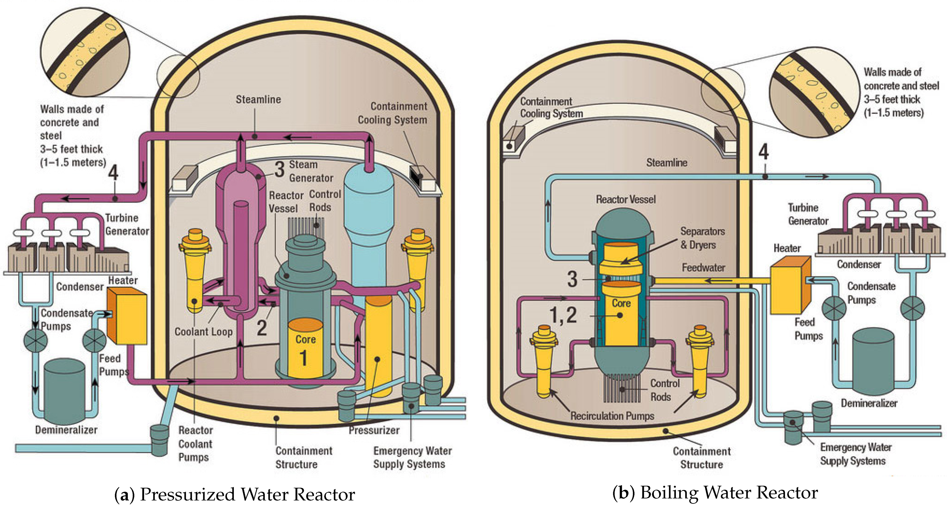
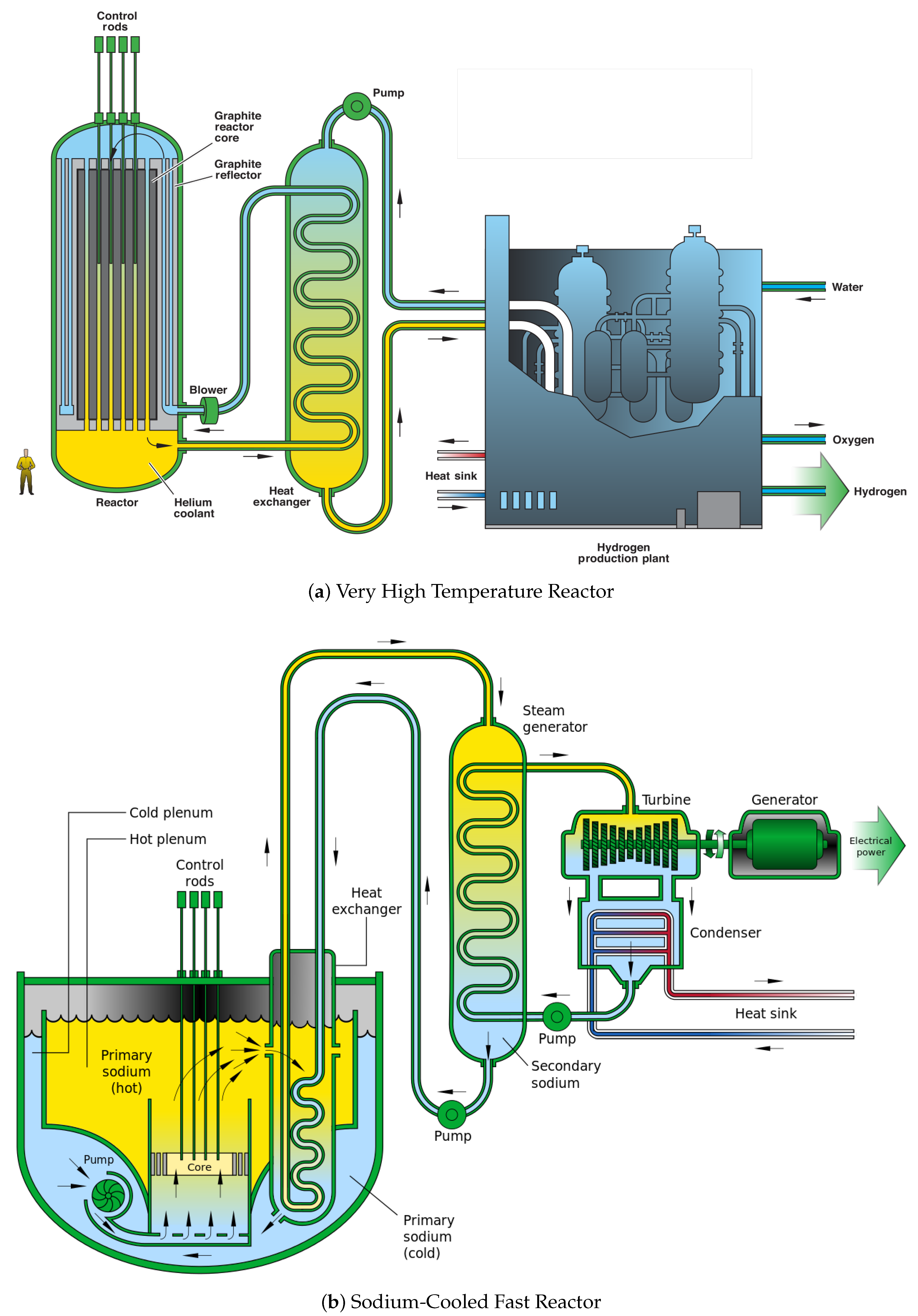
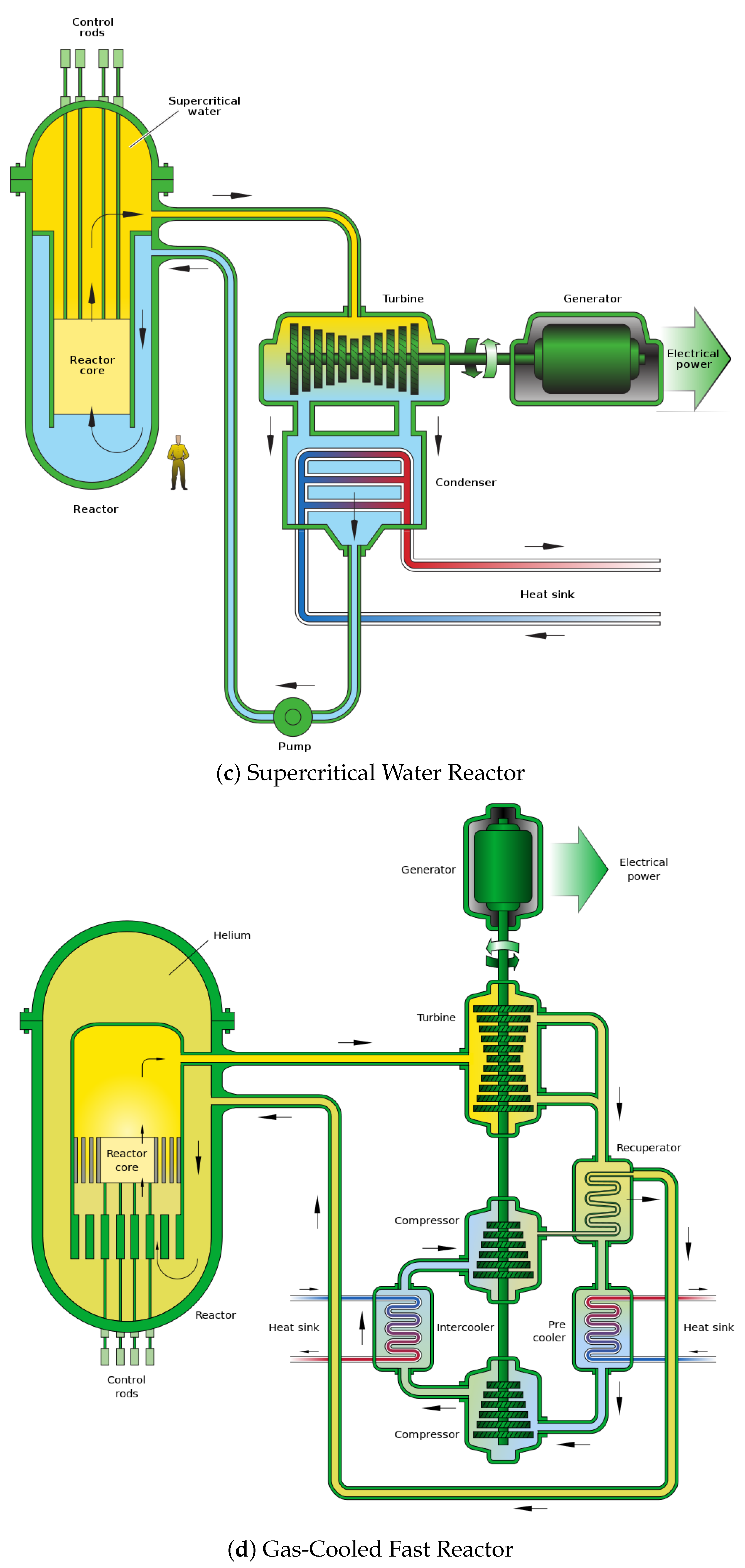
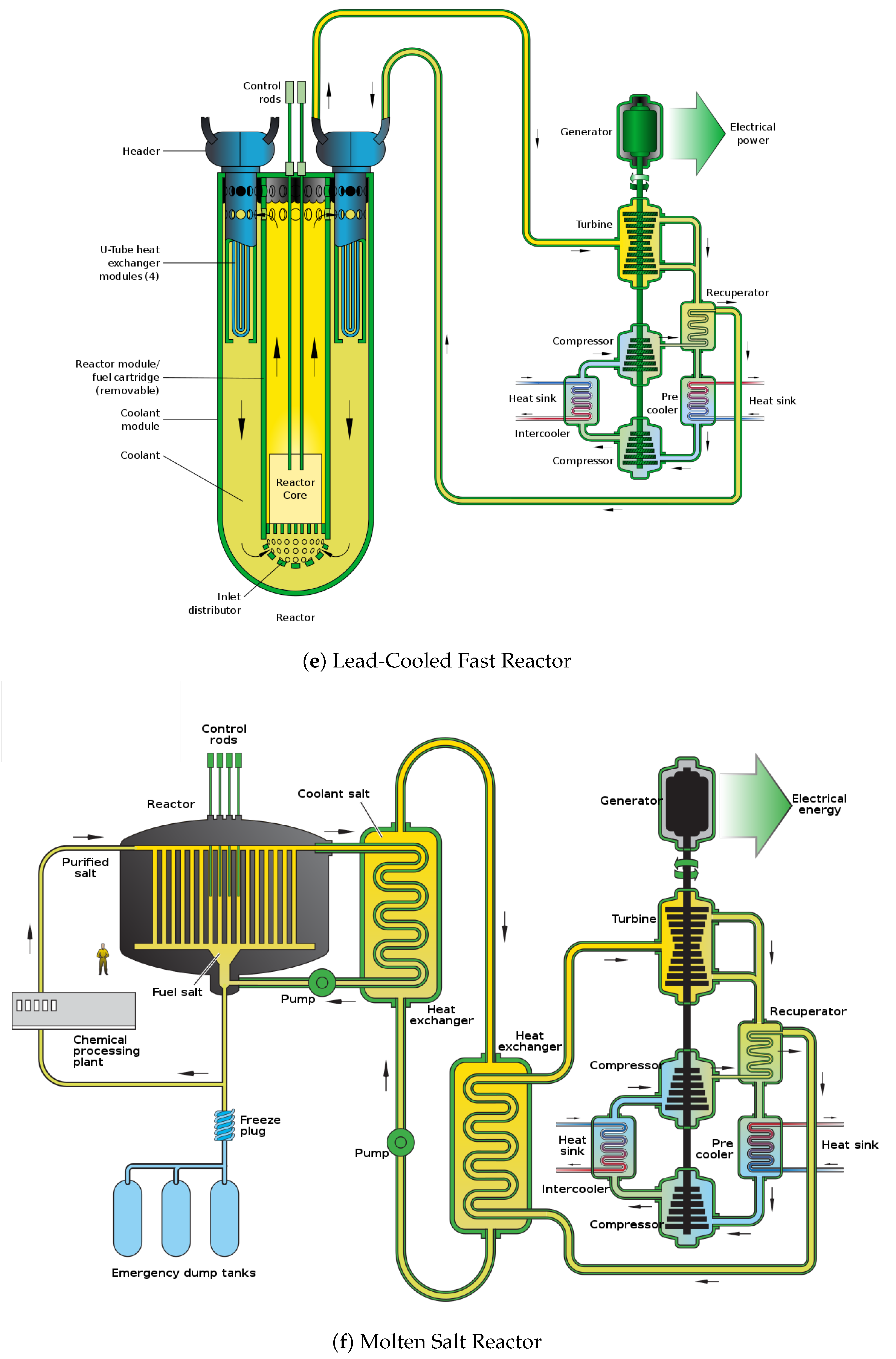
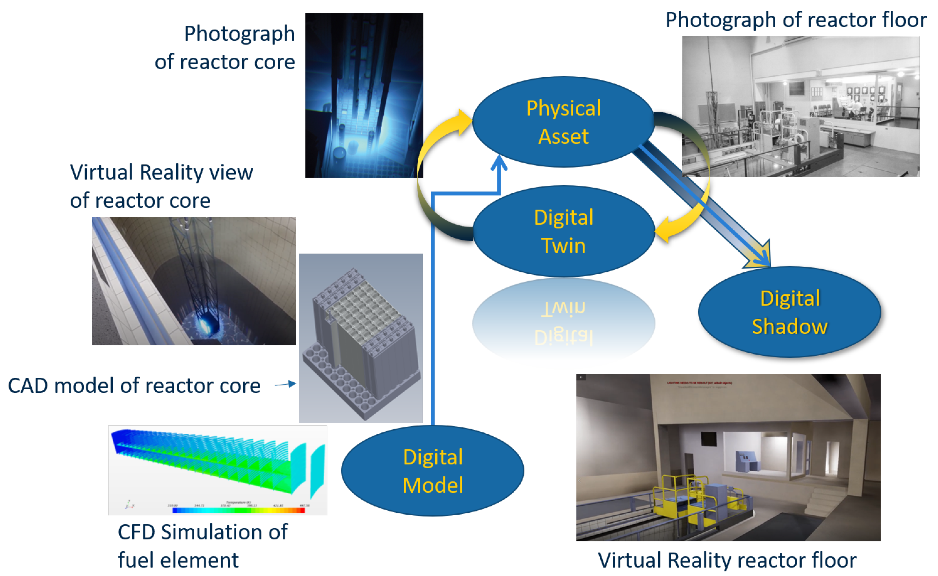
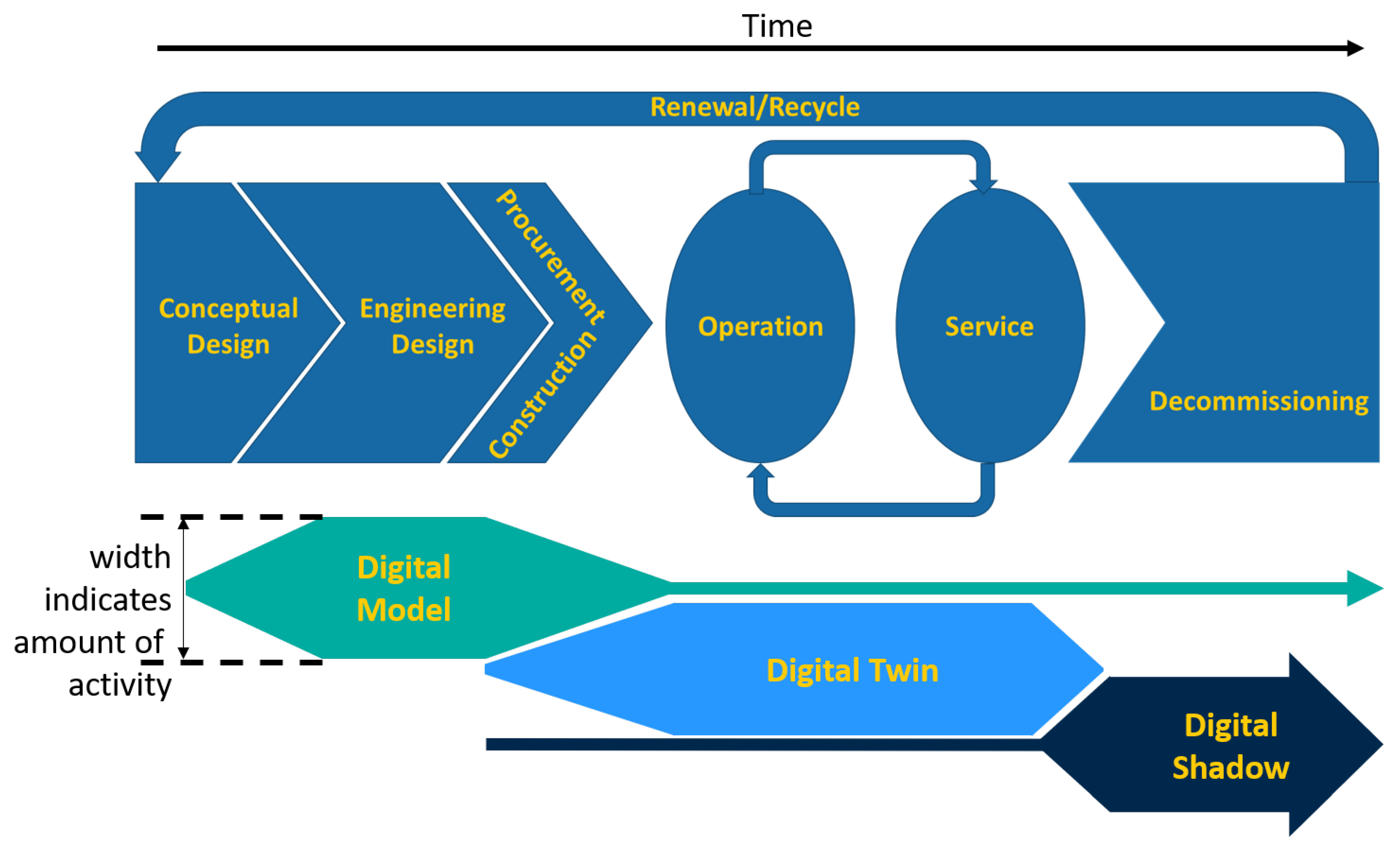
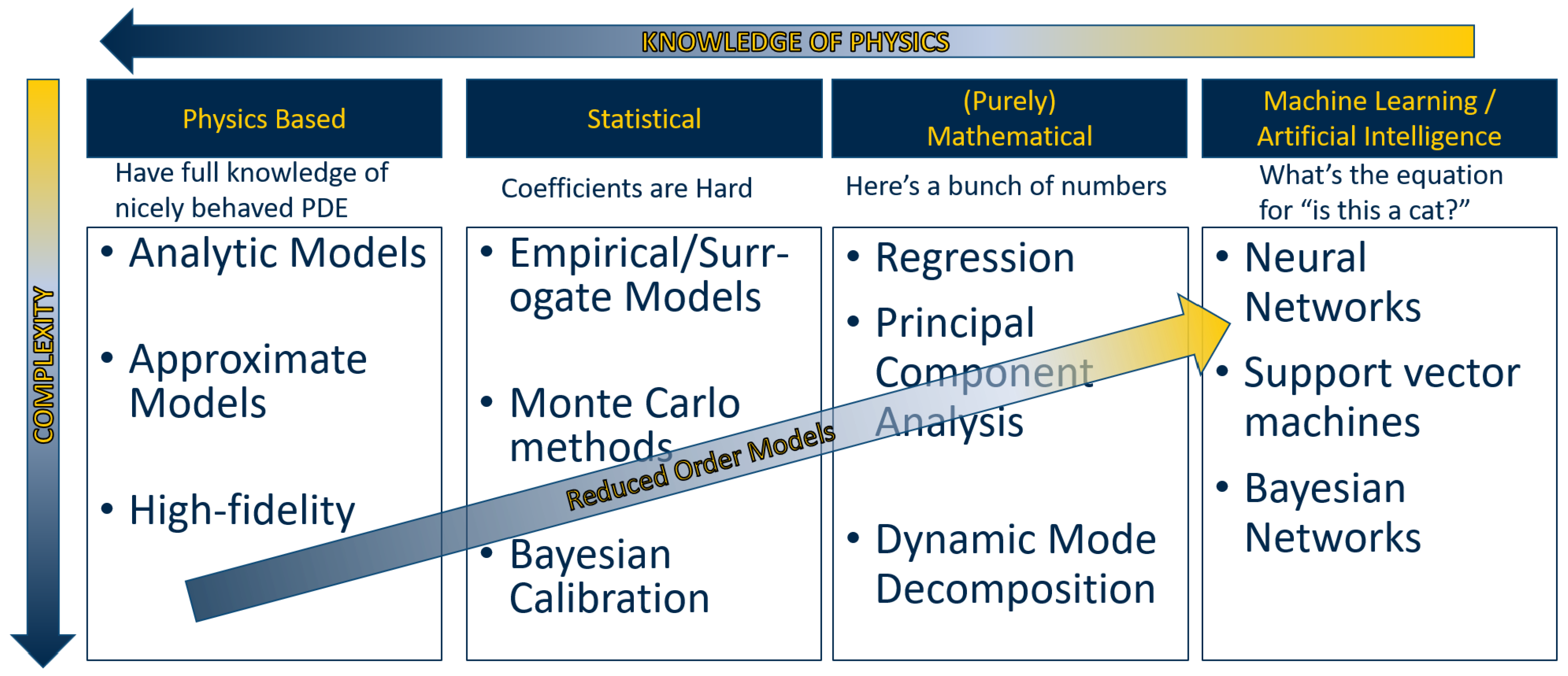
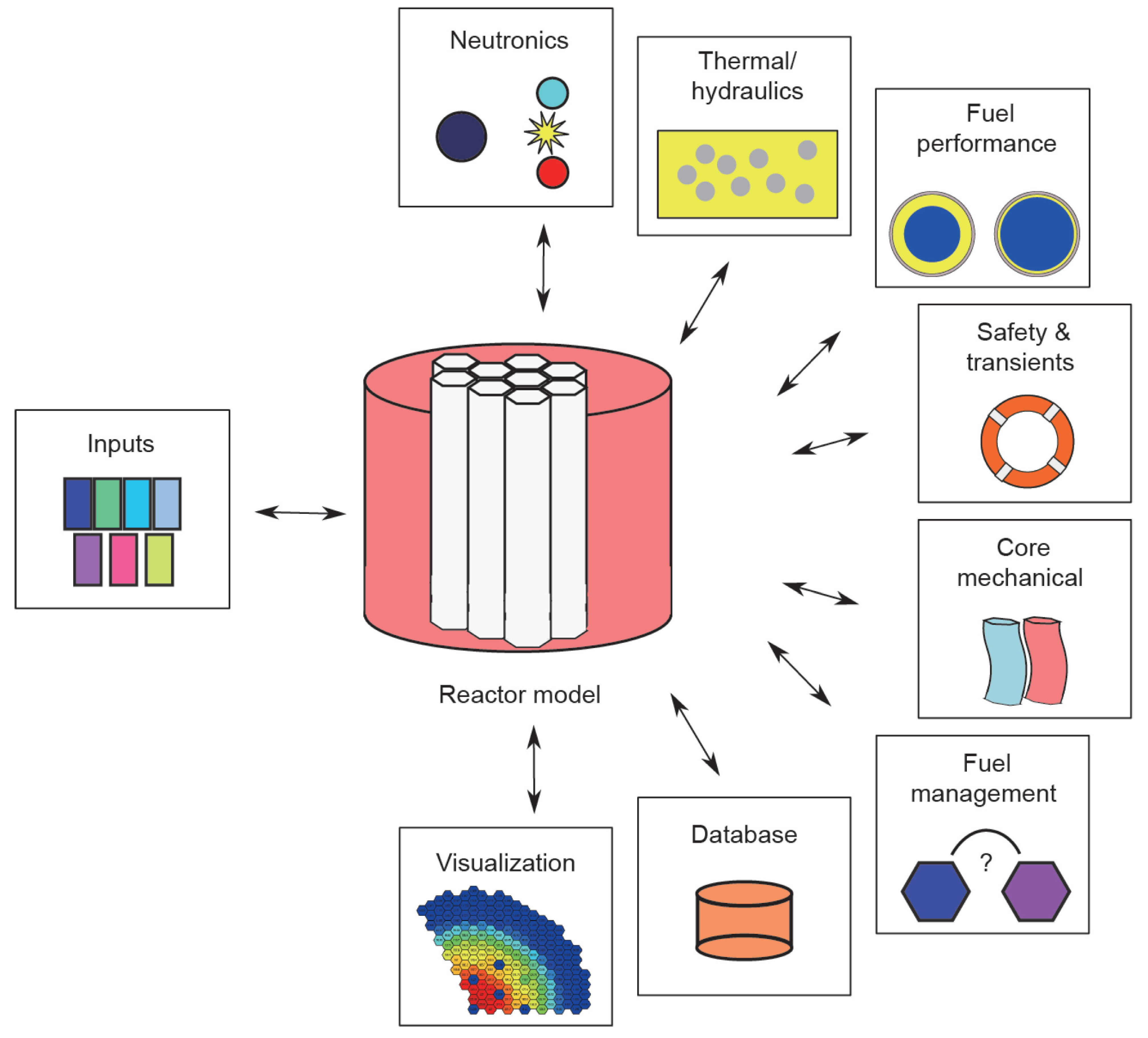
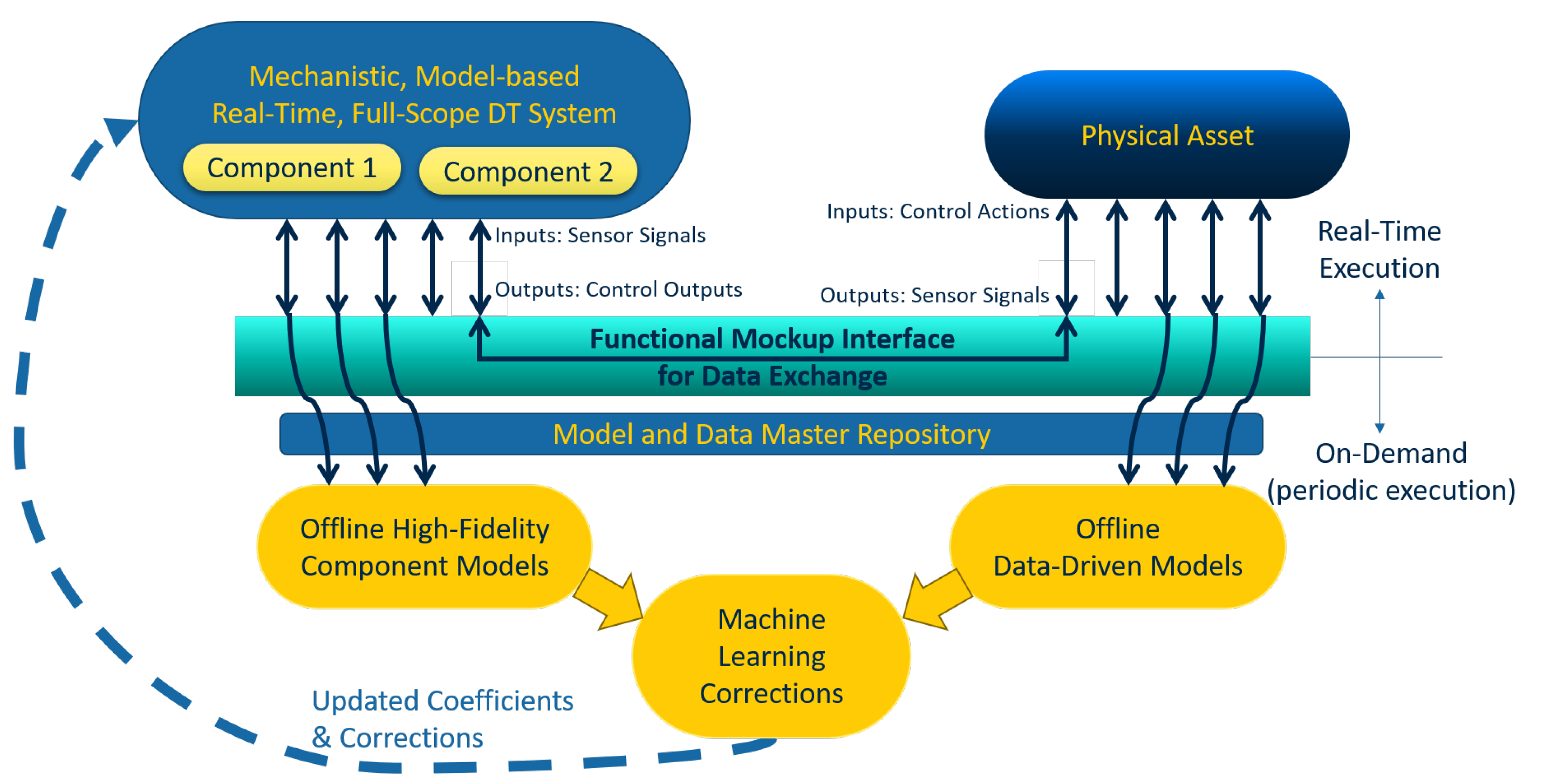
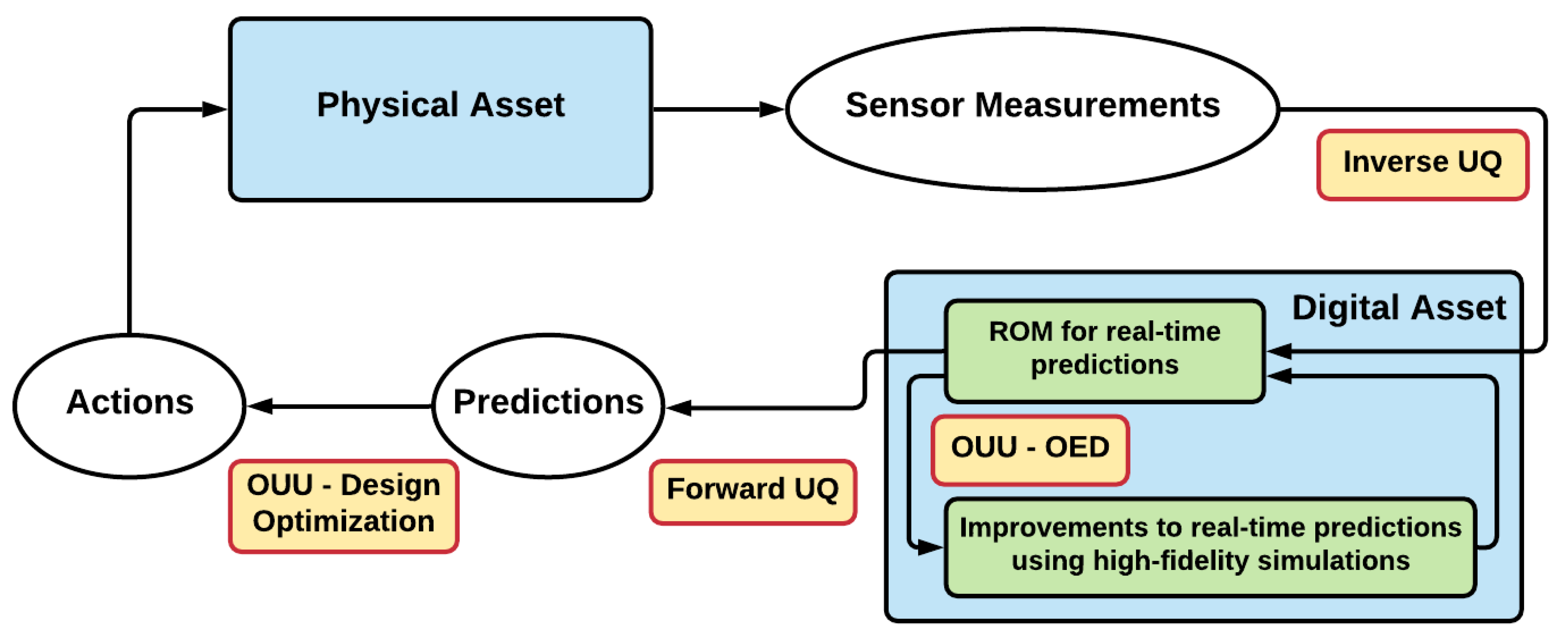
Table 1.
Number of unknowns by type of equation for a real-time, full-scope plant simulator. The -notation indicates order of magnitude. For example, “” in the second row, second column means the “Reactor (x,y)” equations need to solve thousands of unknowns from the discretized differential equations.
| Component | Differential Eqn. | Algebraic Eqn. | Boolean Eqn. |
|---|---|---|---|
| Reactor (x,y) | – | ||
| Reactor Axial | – | ||
| Steam Generator | – | ||
| Turbine | – | ||
| Feed Pumps | – | ||
| Control Systems | – | ||
| Electrical System | – | ||
| Protection System | – | – | |
| Total |
Publisher’s Note: MDPI stays neutral with regard to jurisdictional claims in published maps and institutional affiliations. |
© 2021 by the authors. Licensee MDPI, Basel, Switzerland. This article is an open access article distributed under the terms and conditions of the Creative Commons Attribution (CC BY) license (https://creativecommons.org/licenses/by/4.0/).
Share and Cite
MDPI and ACS Style
Kochunas, B.; Huan, X. Digital Twin Concepts with Uncertainty for Nuclear Power Applications. Energies 2021, 14, 4235. https://doi.org/10.3390/en14144235
AMA Style
Kochunas B, Huan X. Digital Twin Concepts with Uncertainty for Nuclear Power Applications. Energies. 2021; 14(14):4235. https://doi.org/10.3390/en14144235
Chicago/Turabian StyleKochunas, Brendan, and Xun Huan. 2021. "Digital Twin Concepts with Uncertainty for Nuclear Power Applications" Energies 14, no. 14: 4235. https://doi.org/10.3390/en14144235
Note that from the first issue of 2016, this journal uses article numbers instead of page numbers. See further details here.