Shale Reservoir 3D Structural Modeling Using Horizontal Well Data: Main Issues and an Improved Method

Introduction

After over 20 years of the rapid development of hydraulic fracturing in horizontal wells, many shale oil and gas fields exist, most of which are in the United States, Canada, and China (EIA, 2019; IEA, 2019). Horizontal well drilling, as one of the main techniques, opens the door for the commercial shale oil and gas production and has been extensively implemented in the shale play core areas, such as the Barnett Shale in northwestern Texas (Jarvie et al., 2007), the Marcellus Shale in southwestern Pennsylvania (Carter et al., 2011; Wang and Carr, 2013), the Utica-Point Pleasant Shale in eastern Ohio (Shahkarami and Wang, 2017), and the Wufeng–Longmaxi Shale in the Sichuan Basin (Wang, 2015). Data, including wire line logs, formation tops, well location, and well trajectory, in horizontal wells are critical for evaluating the properties of shale reservoirs. For 3D structural modeling, formation tops are the predominant data. However, the horizontal well formation top data have distinct features compared to vertical wells due to the large inclination angle of horizontal wells (Figure 1). The horizontal location of formation tops in one horizontal well is far from each other, while it is the same or similar in vertical wells (Figure 1). This raises new challenges for constructing a 3D structural model of shale reservoirs (Wang et al., 2018a; Qiao et al., 2018; Long et al., 2019; Shu et al., 2020).

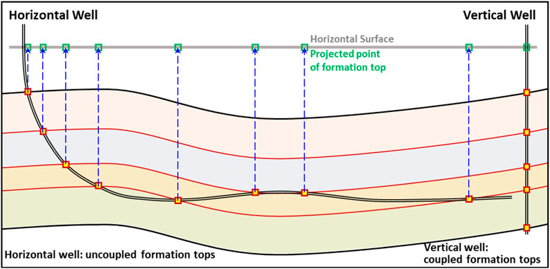
FIGURE 1. Comparison of formation tops and wellbore trajectory characteristics in horizontal wells and vertical wells.

Wang et al. (2018b) developed a method of adding pseudo vertical wells (PVWs) to convert formation tops in each horizontal well to more formation tops in multiple PVWs based on the shale layer thickness. This provides more control points for constructing a high-quality 3D structural model of shale reservoirs. Qiao et al. (2018) used a similar idea to build 3D structural models by transforming horizontal wells into multiple equivalent vertical wells. However, both of them did not provide details of their methods, such as how to add these PVWs and how to transform horizontal wells to multiple vertical wells. Meanwhile, shale thickness data are critical to add formation tops in PVWs, but there is rarely a published method concerning the estimation of shale formation thickness using horizontal well data. In addition, the laterals of horizontal wells are approximately parallel to the formation surfaces and could penetrate through the formation surfaces up and down multiple times, forming a complicated relationship between horizontal wells and formation surfaces. Therefore, it is not surprising that some horizontal wells are located in the wrong formations of the constructed 3D structural model. This causes it necessary to develop a method to effectively detect these errors in the 3D structural model and fix these errors.

The research aimed to present a comprehensive and effective method for 3D structural modeling using data mainly from horizontal wells. In this study, we first discussed the data features in horizontal wells for 3D structural modeling and the main issues using horizontal well data to construct 3D structural models. Then, the developed method for 3D structural modeling using horizontal well data were illustrated in detail and its effectiveness was demonstrated by constructing two 3D structural models of the Wufeng–Longmaxi Shale in the Jiaoshiba area, eastern Sichuan Basin. Finally, an uncertainty source, a level, and a method to reduce these uncertainties were discussed for 3D structural modeling using horizontal wells.

Data Characteristics and Issues

Uncoupled Formation Tops and Abnormal Thickness

The essential purpose of 3D structural modeling is to simultaneously implement spatial interpolation of elevation for multiple formation surfaces to generate a framework for the target formations within the study area. As a result, the spatial distribution of formations, including the formation surface structure and formation thickness, is estimated. In a specific vertical well, all formation tops are in the same or a similar horizontal position (Figure 1). For spatial interpolation using data in vertical wells, the control points from these coupled formation tops are distributed similarly for different formation surfaces within the study area. However, formation tops from horizontal wells are uncoupled, locating at different positions in the same horizontal well. This causes it a challenge to ensure these formation surfaces are coupled with each other because the position distribution of control points can significantly influence the spatial interpolation (Stein, 1999). This influence could be more considerable when the amount of control points is limited. Unfortunately, formation tops are usually scattered in most hydrocarbon reservoirs, and the uncoupled formation tops could cause many severe problems in the 3D structural modeling of shale reservoirs.

The generated formation surfaces using these uncoupled formation tops in horizontal wells are either too close to each other, intersected, or too far away (Figure 2). In the upper part of shale reservoirs, horizontal wells usually intersect with formation surfaces with a large angle (e.g., >70^o) so that formation tops in horizontal wells have a similar distribution feature as those in vertical wells (Figure 2). Meanwhile, a structural map of any formation surfaces, interpreted from either seismic data or other geological sources, could be used as a soft constraint of the spatial interpolation, providing the regional dip angle information. This can mitigate the problem of the abnormal thickness in the upper part of shale reservoirs. Therefore, the issue of abnormal thickness is less serious in the upper part of shale reservoirs. But this issue becomes common in the formations penetrated by horizontal laterals (usually the lower part of shale reservoirs) in which the formation tops, far away from each other laterally, are uncoupled (Figure 2). Although structural maps may exist, using structural maps of formation surfaces as a soft constraint fails to mitigate the abnormal thickness resulting from the uncoupled formation tops.

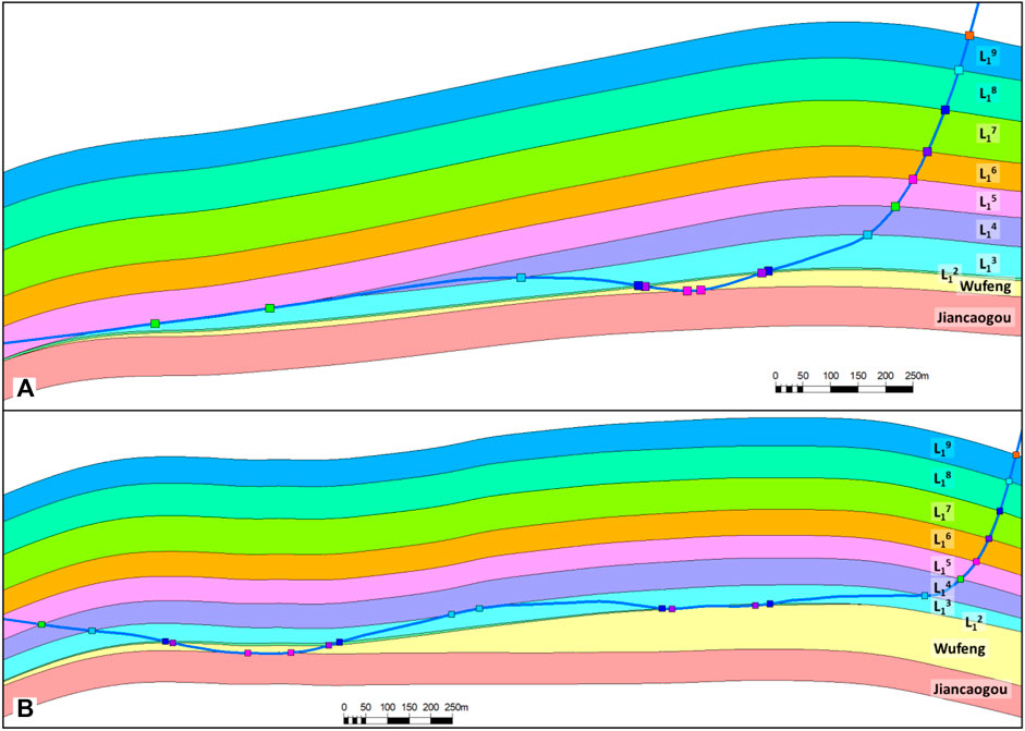
FIGURE 2. The abnormal thickness in the lower part of the 3D structural model of the Wufeng–Longmaxi Shale reservoir in the Jiaoshiba area. (A) Cross section along the well JY-a; (B) cross section along the well JY-b.

The Large Wellbore Inclination and Incorrect Landing Formation

The formation tops divide the well trajectory into multiple segments and each segment lands in a specific formation, which is named landing formation in this research. The landing formation data are along well trajectory, including the location (X and Y) and formation ID (Table 1). In an individual vertical well, the horizontal location of landing formations is the same as or similar to their formation tops (Figure 1). Therefore, the formation tops in vertical wells usually ensure the vertical wells landing in the correct formations in the 3D structural model. However, landing formations and formation tops in horizontal wells are usually at different horizontal locations. It is common that some segments of horizontal wells land in the incorrect formation in the constructed 3D structural model, especially in the segments with relatively large inclination (e.g., >70^o) and limited control from formation tops. In 3D structural modeling for shale reservoirs, it is critical to ensure all well segments land in the correct formation. Therefore, the landing formation data serve as a soft constraint to check errors within the 3D structural model and provide the necessary data to fix these errors.

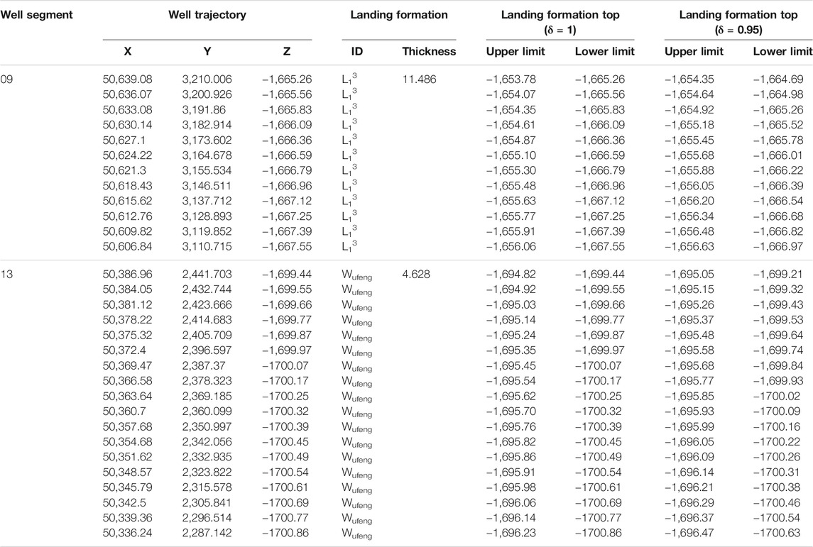
TABLE 1. Example of Landing Formation Data and the Inferred Elevation Range of the Landing Formation Top. The data in gray-filled cells are for the added pseudo vertical wells.

Methodology

To construct a high-quality 3D structural model for shale reservoirs using horizontal well data, we need to deal with the uncoupled spatial interpolation and the incorrect landing formation. For the uncoupled spatial interpolation of multiple formation surfaces, our approach is to convert the uncoupled formation tops to the coupled formation tops by adding pseudo vertical wells at formation top data (PVW-As) in all horizontal wells (Wang et al., 2018b; Figure 3). The elevation of formation tops in these PVW-As can be calculated using the elevation of the formation top at the intersection point and the thickness of shale layers (Figure 3A). The uncoupled formation tops in horizontal wells become coupled after adding formation tops in these PVW-As for all formations, fixing the uncoupled spatial interpolation. Now, the problem is that the thickness of shale layers is unknown. Therefore, in this method, the key is to estimate the thickness of all shale layers.

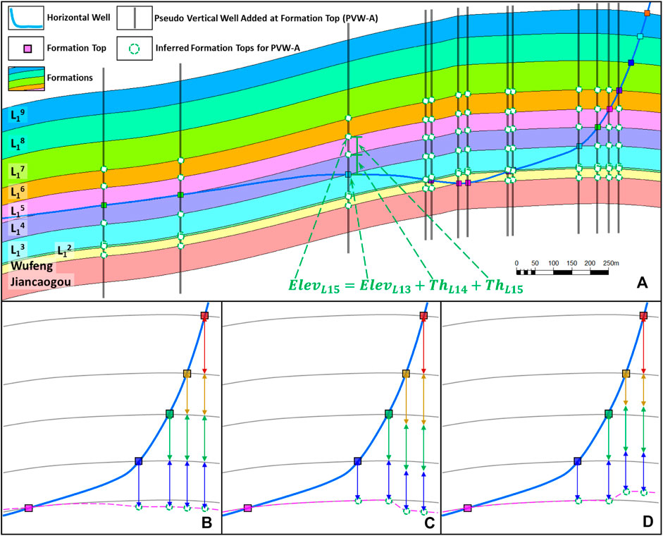
FIGURE 3. Pseudo vertical wells added at formation tops (PVW-A) for the well JY-a in the Jiaoshiba area, Sichuan Basin (A) and the effects of shale layer thickness on formation top elevation calculation (B–D).

In this research, one part of our improved method is to estimate the thickness of shale layers by balancing the dip angle change and the shale thickness change. This method involves two items: the initial thickness of shale layers and the dip angle change of a key surface. The key surface should have strong responses in wire line logs and seismic data, for example, the Wufeng base in the Jiaoshiba area. First, an initial thickness of all shale layers should be estimated from the formation tops in vertical wells. Within a relatively small area (e.g., a well pad), we can assume that the shale layer thickness is constant or has little change (Wang et al., 2018a), so the formation tops in vertical wells can usually give a reasonable estimation of the initial shale thickness. In a relatively large area, the shale thickness could change significantly, so does the dip angle of the key surface. If only limited vertical wells exist, their formation tops are usually insufficient to give a reasonable estimation of the initial shale thickness. Therefore, we developed an iterative process to repeatedly update the shale thickness and the structural map of the key surface by balancing the dip angle and shale thickness. In detail, the thickness contour map using vertical well data only is used to calculate the elevation of the key surface at all PVW-As, and then a smoothed structural map of the key surface was generated to calculate the shale thickness at all PVW-As, which were used to make their smoothed contour maps. This process could be repeated several times, and these smoothed thickness contour maps were used as the initial thickness in the study area.

The initial thickness of shale layers has two main functions: 1) to estimate the actual shale thickness by adjusting the initial thickness, and 2) to set the thickness change threshold, which is a percentage of the initial thickness. Again, the elevation of the key surface at all PVW-As was calculated using the initial thickness to generate its structural map. The dip angle change of the key surface at all PVW-As was calculated to detect any value larger than the dip angle change threshold. As shown in Figures 3B–D, the large dip angle change usually results from the large differences between the initial and actual thickness of shale layers. Therefore, the shale thickness should be decreased or increased within a range, the thickness change threshold (e.g., 10% of the original formation thickness), to reduce the dip angle change (see Supplementary Appendix for more details). This process continues until all dip angle changes are less than the dip angle change threshold. We developed a VBA program to achieve this process automatically. Finally, the TVTs estimated from all PVW-As and vertical wells together provide a larger dataset to analyze the distribution of formation thickness inside the area statistically. All abnormal TVTs that exist inside the study area should be double-checked.

The incorrect landing formation errors in the 3D structural model can be solved by adding a PVW for each well segment with an error (PVW-B; Figure 4A). The PVW-B is usually added at the middle of the well segment with an error. Different from PVW-As, a PVW-B intersects with the horizontal well within a specific formation and the relative position of the intersection point in this formation is unclear. Therefore, there is no enough data to determine the elevation of any formation tops in PVW-Bs, but we can determine the elevation range of formation tops in PVW-Bs (Figures 4B,C). Given that the elevation of the intersection point between a PVW-B and horizontal well is ELEV and its landing formation thickness is TH, the formation top elevation of the intersection point’s landing formation in the PVW-B must be larger than ELEV and smaller than ELEV + TH (Table 1; Figures 4B,C). The elevation range of a formation top that cannot be directly used as an input of the spatial interpolation should be converted to an exact elevation value. A straightforward method is to arbitrarily use the mid-point or a random point within the elevation range, but it is prone to cause large dip angle change at the location of PVW-Bs, especially when PVW-Bs are close to any other wells (horizontal wells, PVW-As, or other PVW-Bs). In order to minimize these dip angle changes, a better strategy is to use the point within the elevation range and closest to the formation surfaces at the location of PVW-Bs. This closest point is either the lower limit (Figure 4B) or the upper limit (Figure 4C) of the elevation range. This approach results in the slightest change of the current 3D structural model. Besides, this research introduced a confidential constant δ (0.5≤δ ≤ 1) to re-calculate the elevation range as ELEV+(1−δ)TH to ELEV + δTH. This confidential constant reduces the elevation ranges, offers more options for 3D structural modeling (Table 1), and can fit the real geological situation better. After determining the formation top elevation of the intersection point’s landing formation, all formation tops in PVW-Bs can be calculated using the TVT of shale layers, and the 3D structural model can be reconstructed. This process should continue until no more errors exist in the 3D structural model.

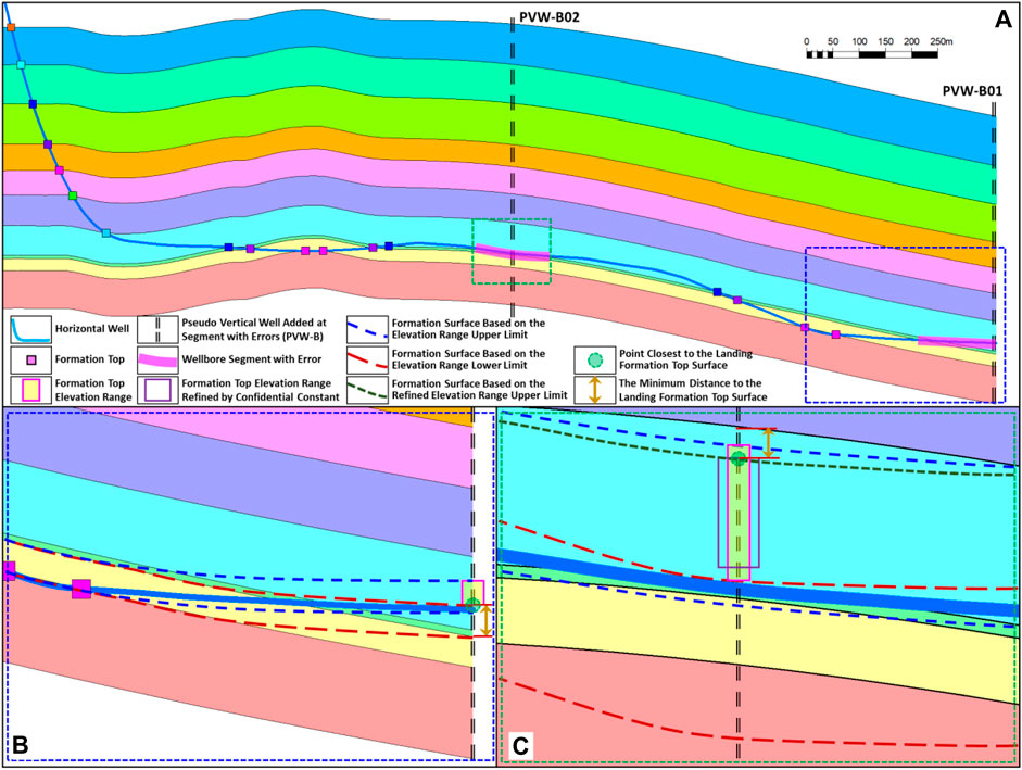
FIGURE 4. Pseudo vertical wells added for the well segments with the incorrect landing formation (PVW-B) and the formation top of the intersection points landing formation added for PVW-Bs. (A) Well JY-b and the well segments with error; (B) elevation range and the formation top using its lower limit; and (C) elevation range refined by confidential constant and formation top using its upper limit. The two dash rectangles indicate the location of Figures 4B,C.

A generalized workflow of this method is shown in Figure 5, including adding PVW-As, iteratively updating TVTs based on dip angle changes, detecting all incorrect landing formations, and adding PVW-Bs. This workflow can be revised in terms of the data features in a specific study area.

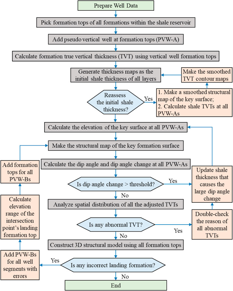
FIGURE 5. A generalized workflow to build a 3D structural model for shale oil and shale gas fields using horizontal wells.

Results

Two case studies using data of the Wufeng–Longmaxi Shale in the Jiaoshiba area, eastern Sichuan Basin, have been implemented to validate the method in this research (Table 2). The first case is to build a 3D structural model for the JY-1 district, which was located in the northern Jiaoshiba area. This area includes eight horizontal wells and five vertical wells (one inside and four outside the JY-1 district). This case represents a typical situation to build a well pad scale 3D structural model of shale reservoirs. The second case is to construct a 3D structural model for the whole Jiaoshiba area, including 283 horizontal wells and eight vertical wells. We assumed that the seismic data were only accessible for the second case to enlarge the differences between the two cases. Besides, we only constructed the 3D structural model of the lower six shale layers (Figure 4A) for the first case in which all the eight horizontal wells targeted the lower part of the Wufeng–Longmaxi Shale. In contrast, all the nine shale layers (Figure 4A) were analyzed in the second case.

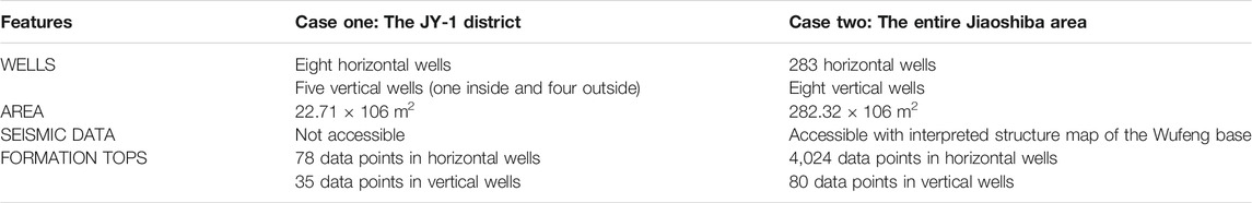
TABLE 2. Data features of the two cases in the Jiaoshiba area, eastern Sichuan Basin.

Well Pad Scale 3D Structural Modeling: The JY-1 District

This study case represents a situation that we need to construct a 3D structural model of one or two well pads surrounded by many vertical wells. This situation is common because many shale plays are located within conventional oil and gas fields, such as the Marcellus Shale in the Appalachian Basin, the Eagle Ford Shale in the Permian Basin, and the Qingshankou Shale in the Songliao Basin. The development of conventional oil and gas has drilled a significant number of vertical wells, which can provide lots of constraint points to estimate the shale thickness. Meanwhile, when the study area is relatively small, the available vertical wells can give a reasonable estimation of shale thickness, assuming that shale formations do not or only gradually change within a small area (Wang et al., 2018b). Therefore, the data in vertical wells can make a reliable estimation of shale thickness with relatively low uncertainty, simplifying the process of 3D structural modeling.

In this case, there are a total of 94 formation top data points for the six layers within the Wufeng–Longmaxi Shale, including 87 points in the eight horizontal wells and 35 points in the vertical wells. A PVW-A was added for each formation top in the horizontal wells, adding 87 PVW-As in total (Figure 6). The seven formation tops in the vertical well JY-1 were used to calculate the actual vertical thickness (TVT) of the six shale layers at well JY-1, which were used as the TVTs of the six shale layers in the entire JY-1 district. Therefore, we can calculate the Wufeng base elevation at all PVW-As using the shale layer thickness and formation tops in horizontal wells (Figure 3). As a result, the amount of control points for Wufeng base mapping was significantly increased from 11 log-interpreted formation tops in horizontal and vertical wells to 88 points (Figure 6). The structural map of Wufeng base is shown in Figures 6, 7. Compared to the 3D structural model along the horizontal wells JY-a and JY-b, in Figure 2, the 3D structural model using our improved method has a much better quality.

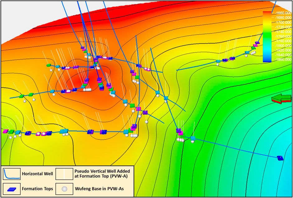
FIGURE 6. Log-interpreted formation tops and the pseudo vertical wells added at these formation tops (PVW-As) with the inferred formation top of the Wufeng base. The structural map is the Wufeng base generated using the formation top in all wells, including the horizontal wells, the vertical wells, and PVW-As.

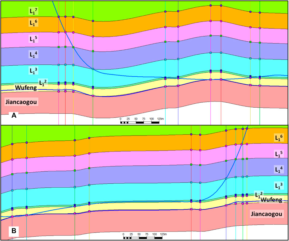
FIGURE 7. Cross sections of wells JY-b and JY-c with the inferred formation tops in PVW-As. The blue X and the blue curve represent the formation top for the Wufeng base that was calculated using the TVTs from the well JY-1 and the Wufeng base structural map made from these inferred formation top. The color-filled squares in the PVW-As are the formation tops after adjusting the TVTs for shale layers based on the dip angle change threshold of 2.5^o.

In the structural map of the Wufeng base, the dip angle significantly changed at the location of some PVW-As (Figures 7, 8). The dip angle and curvature contour maps (Figure 8) helped view and summarize these dip angle changes. This mainly resulted from the significant differences between the initial thickness and actual thickness of shale layers. We mitigated the dip angle change by altering the TVTs at the location of these PVW-As automatically using our developed VBA program. For example, as shown in Figure 7, the dip angle change of the Wufeng base surface was reduced by increasing the thickness of L₁⁴ at well JY-b and JY-c. This increased the variation of shale thickness but reduced the dip angle changes. Therefore, we used the dip angle change threshold and thickness change threshold to limit the dip angle change and TVT change within an acceptable range. Using different values of the two thresholds, for example, the estimated thickness of the Wufeng Formation was different (Figure 9). The largest thickness variation occurred when setting dip angle change threshold as 1.5^o and thickness change threshold as 30% (Figure 9). This indicated that, in order to limit the dip angle change to less than 1.5^o, the thickness of the Wufeng Formation should be significantly increased or decreased. Also, the Wufeng Formation thickness was similar for all the six cases that the dip angle change threshold was set to 2.5^o and 3.0^o (Figure 9). In this research, based on the thickness change of all the six layers, we used the dip angle change threshold of 2.5^o and thickness change threshold of 10% to estimate the thickness of the six shale layers (Figure 10). Within this small area, it is a little difficult to analyze the trend of thickness change statistically, so we directly used these TVTs to calculate the elevation of formation tops in all PVW-As (Figure 7).

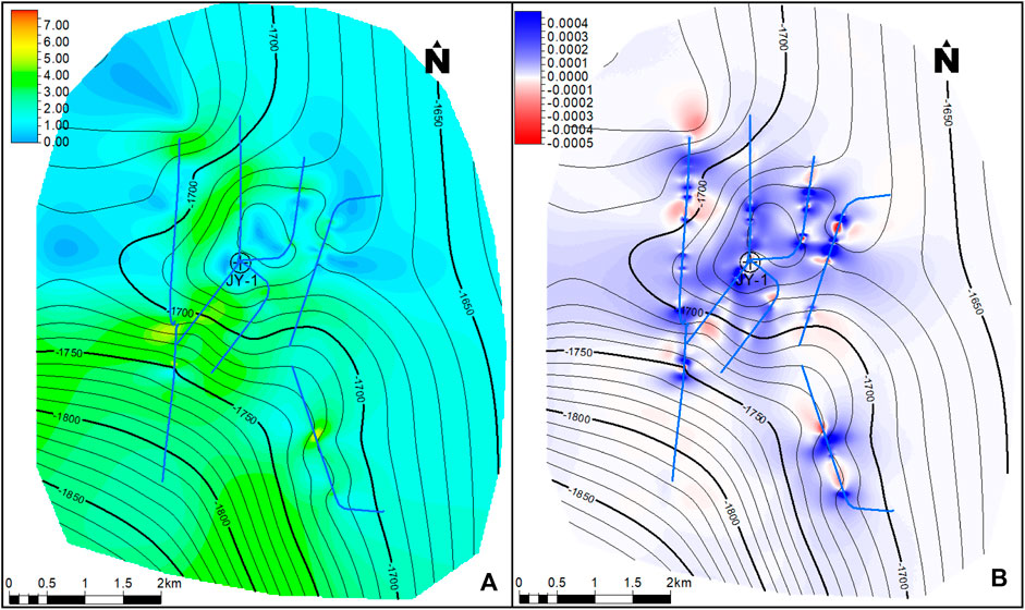
FIGURE 8. The contour map of the dip angle (A) and curvature (B) of the Wufeng base surface that was made from the inferred formation top using shale layer TVTs from the vertical well JY-1.

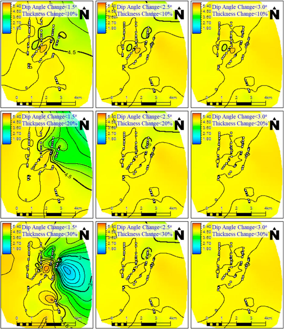
FIGURE 9. Isopach maps of the Wufeng Formation in the JY-1 district after adjusting its TVT at the location of PVW-As using different dip angle change thresholds and thickness change thresholds. The white-filled squares represent the location of formation tops in the vertical and horizontal wells.

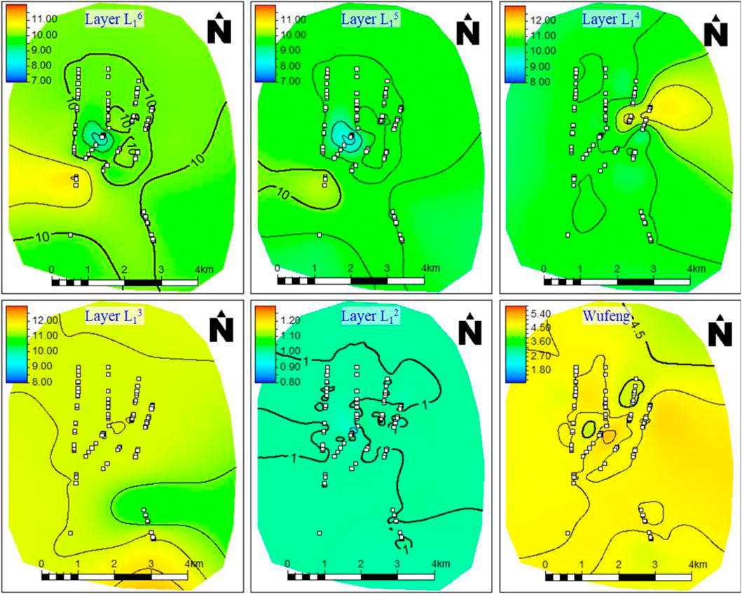
FIGURE 10. Isopach maps of the six shale layers in the JY-1 district after adjusting their TVTs using dip angle change threshold of 2.5° and thickness change threshold of 10%. The white-filled squares represent the location of PVW-As.

The formation tops in all horizontal wells, the vertical well, and PVA-As were used to build the 3D structural model in the JY-1 district. However, we detected errors in six segments in four horizontal wells. Figures 11A,B showed an example of the errors in well JY-b. It is worth pointing out that, to check errors in all horizontal wells quickly, we extracted the landing formation information from the constructed 3D structural model and compared it with the landing formation determined from formation tops using the VBA program (Figure 11B). For each well segment with error, we added one pseudo vertical well (PVW-B) at the middle of the well segment and calculated their formation tops with a confidential constant of 0.95 (Figure 11C). All errors were removed after adding these PVW-Bs and their formation tops.

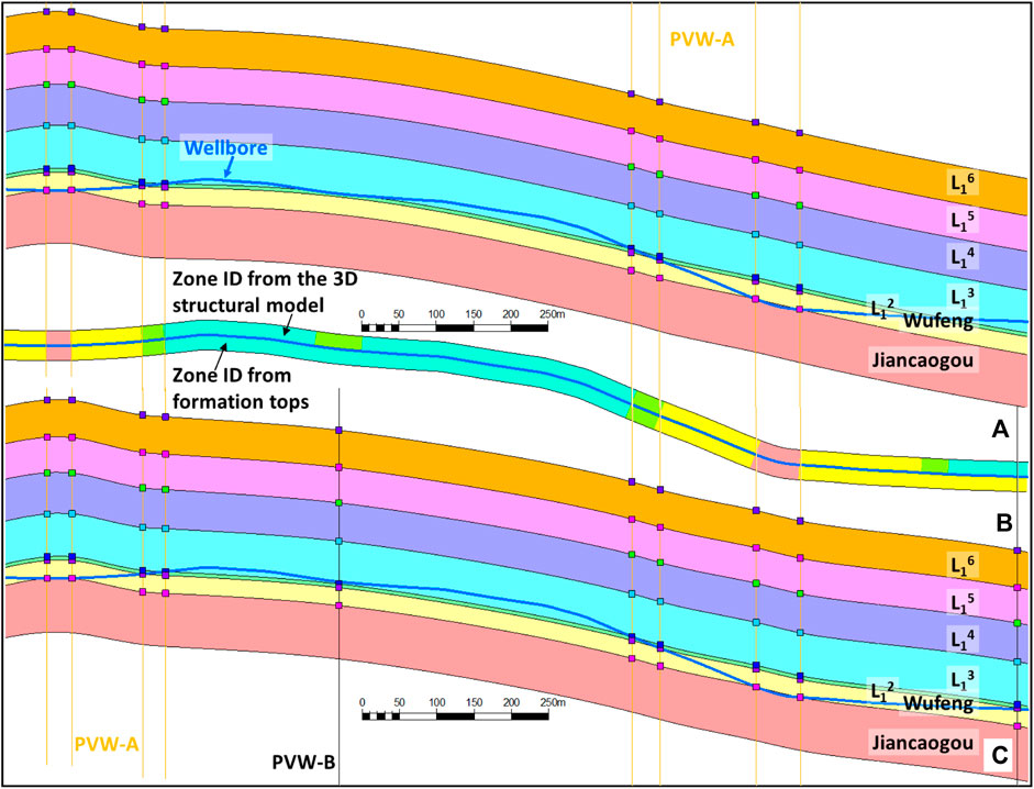
FIGURE 11. Examples of errors in the 3D structural model (A–B) and the pseudo vertical wells added to fix these errors (PVW-B) (C).

Regional/Basin Scale 3D Structural Modeling: The Jiaoshiba Area

The Jiaoshiba area was much larger than the JY-1 district, with 283 horizontal wells. The data available for 3D structural modeling are summarized in Table 1. Similar to the first case, we added a PVW-A at each of all the 4,024 formation tops in the horizontal wells. The structural map of the Wufeng base interpreted from 3D seismic data was available (Figure 12A) and used as the second input for making the structural map of the key surface. Besides, within this relatively larger area, both the formation surface dip angle and thickness had a larger range. This caused two major differences from the first case in estimating the thickness of shale layers.

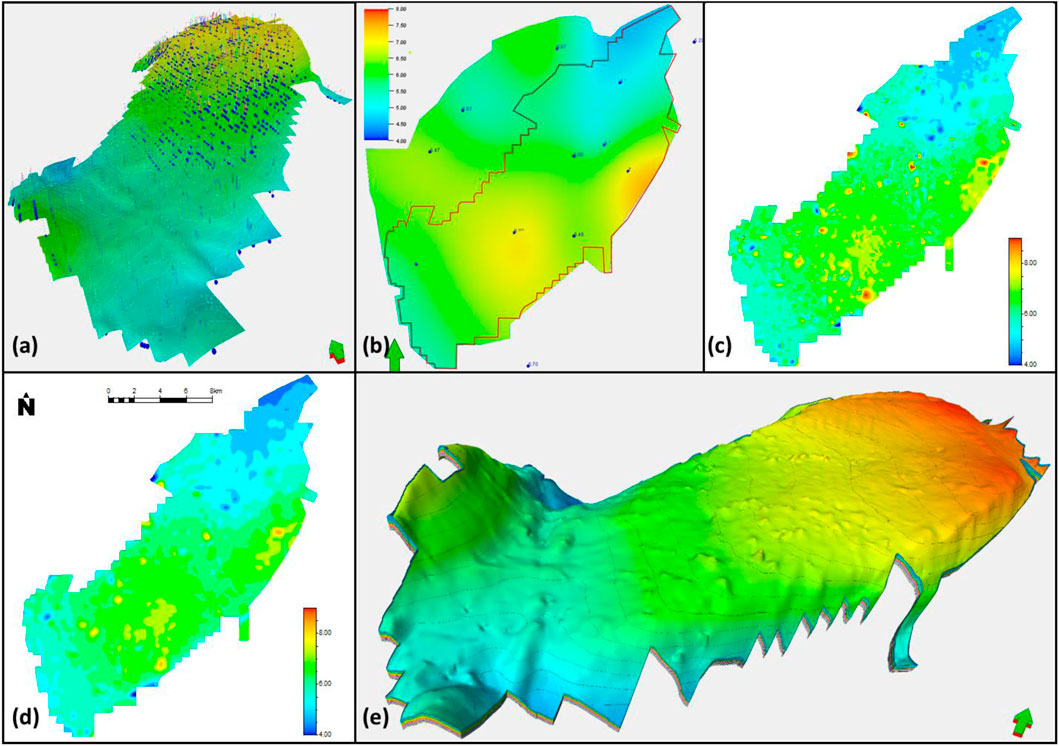
FIGURE 12. (A) Seismic-interpreted structural map of the Wufeng base with the inferred Wufeng base elevation at PVW-As; (B) the Wufeng Formation TST contour map generated by formation top data in vertical wells; (C) the Wufeng formation TST contour map generated by formation top data in PVW-As and vertical wells; (D) the smoothed Wufeng formation TST contour map; and (E) the 3D structural model of the Jiaoshiba area in the eastern Sichuan Basin.

The first one was to deal with the differences between the true stratigraphic thickness (TST) and the true vertical thickness (TVT). When the dip angle is large, for example, ∼20^o in the marginal area of Jiaoshiba (Figure 12A), the TST is much different from TVT. Since the TVTs are affected by formation dip angle, it is better to use TST to analyze the distribution features of shale layers. In the Jiaoshiba area, the initial value of formation dip angle was estimated from the seismic-interpreted structural map of the Wufeng base (Figure 12A), and the formation tops in vertical wells were used to generate the TST contour maps of all shale layers (Figure 12B). Then, the dip angle of the Wufeng base surface, formation tops in horizontal wells, and the TST contour maps were used together to calculate the Wufeng base elevation at all PVW-As (Figure 12A).

The second difference was to estimate the initial thickness of shale layers using an iterative process (Figure 5). Within the small area of the JY-1 district, the thickness of each shale layer was considered as constant and set to the value in the vertical well JY-1. However, in the relatively larger area of the entire Jiaoshiba area, data in the limited vertical wells failed to give a high-quality estimation of shale layer thickness, especially in the areas far away from the vertical wells. Therefore, we should also take the thickness information extracted from horizontal wells into consideration by the iterative process. First, the TST data that were calculated at all PVW-As (Figure 12C) were used to re-evaluate the distribution features of shale layer thickness by smoothing the TST contour maps (Figure 12D). Then, the elevation of the Wufeng base at all PVW-As was updated again, and its dig angle was re-calculated, which was used to calculate the TSTs at all PVW-As again. Therefore, the dip angle of the Wufeng base, the TSTs at all PVW-As, and the smoothed TST contour maps were repeatedly calculated in three iterations in this research to provide a better estimation of the initial shale thickness.

The estimated initial shale thickness of shale layers was utilized to calculate the elevation of the key surface Wufeng base. Then, the dip angle change threshold and the thickness change threshold were set to 2.5^o and 15%, respectively, to balance the dip angle change of the Wufeng base and thickness change of the nine shale layers. Finally, these data were combined to create a 3D structural model of the entire Jiaoshiba area, in which we found errors in 118 segments in 69 horizontal wells. Therefore, we added 118 PVW-Bs to remove all the errors in the 3D structural model. Figure 12E showed the final version of the 3D structural model using the formation tops in vertical wells, horizontal wells, PVW-As, and PVW-Bs.

Discussion

Uncertainty is an essential component of 3D geological modeling, and it is critical to understand and estimate the uncertainties in geological models (Lelliott et al., 2009; Wellmann et al., 2014; Krajnovich et al., 2020; Liang et al., 2021). Compared to 3D structural modeling for conventional reservoirs, both data and methods were different in 3D structural modeling for shale reservoirs. Therefore, it is necessary to discuss the uncertainty in the 3D structural model of shale reservoirs. In this research, we classified the uncertainty into two groups: data-associated uncertainty and process-associated uncertainty.

Data-Associated Uncertainty

According to the features of data used for 3D structural modeling of shale reservoirs, we grouped all the data into five types and recognized their uncertainty to three levels. Well location and trajectory data are considered in the first group with the first-level uncertainty, also called hard data. They together define the spatial position of all well-related data. Uncertainty of well location and trajectory results from data measurement due to equipment and human error. In general, this uncertainty should be the least compared to all other data. Compared to well location, it is more challenging to measure the well trajectory in the underground (Zhou, 2015; Liu, 2018; Shtuka et al., 2018), and, as a result, the uncertainty of well trajectory should be higher than well location. Meanwhile, the uncertainty of well trajectory could be more significant when close to well toe since errors will accumulate along the wellbore.

Formation tops are interpreted from wire line logs and their locations are determined from well location and trajectory. Therefore, the uncertainty of formation tops is affected by the uncertainty of log data (mainly gamma-ray log, resistivity log, and measured depth), well location, well trajectory, and the performance of formation top interpretation. In general, the uncertainty of formation tops is larger than well location and trajectory but smaller than the other data. This research considered the formation tops interpreted from well logs as the second group with the first-level uncertainty. In addition, as for the performance of formation top interpretation, it is usually easier to recognize the formation tops with clear lithology changes, such as the base and top surface of the shale reservoir, and consequently, the uncertainty of formation tops with stronger log response is smaller. In addition, the uncertainty of formation tops in horizontal wells is usually more considerable than them in vertical wells because it is much more challenging to interpret formation tops in horizontal wells, especially in the lateral segments due to the logging process and formation repetition (Passey et al., 2005; Griffiths et al., 2012; Maggs et al., 2014; Wang et al., 2018a).

The inferred formation tops in PVW-As are considered the third group with the second-level uncertainty, which has a relatively larger uncertainty than formation tops interpreted from wire line logs. This uncertainty is primarily affected by the estimated thickness contour maps of shale layers and the interpreted formation tops. The relatively high uncertainty of thickness contour maps is the main reason for the high uncertainty of inferred formation tops in PVW-As. In order to reduce this uncertainty, the estimation of the thickness contour maps should be improved, such as the iterative process to estimate the thickness distribution in the entire Jiaoshiba area (Figures 12B–D). The inferred formation tops in PVW-Bs are considered the fourth group with the third-level uncertainty, also called soft data, due to their high uncertainty. In fact, we can only determine the elevation range of formation tops in PVW-Bs. This elevation range is strongly associated with the thickness of the landing formation of the intersection point between the horizontal well and PVW-B (Figure 4 and Table 1). A feasible way to reduce this uncertainty is to recognize more shale layers within the shale reservoir to reduce the thickness of each shale layer. Besides, refining the relative vertical position of the intersection point within the landing formation can also reduce this uncertainty.

Structural map interpreted from seismic data is considered the fifth group with the third-level uncertainty (soft data). Seismic data have a relatively low vertical resolution of seismic data and the high uncertainty of velocity model to convert seismic data from time to depth domain (Fomel and Landa, 2014; Donahoe and Gao, 2016; Pinto et al., 2017). This uncertainty should be much larger than well location and trajectory, formation tops interpreted from well logs, and formation tops inferred in PVW-As. Therefore, seismic-interpreted structural maps are usually used as a soft constraint to build the 3D structural models.

Process-Associated Uncertainty

In addition to the data itself, the method to process these data can also significantly affect the uncertainty within the 3D structural models. Three major processes affect the uncertainty of 3D structural modeling using horizontal well data. The first one is the initial thickness of shale layers used to calculate the elevation of the key surface (e.g., the Wufeng base) at all PVW-As since the adjustment of shale thickness is based on the initial thickness. The effect of the selected initial thickness of shale layers is small if the study area is relatively small but becomes serious within a relatively large area (e.g., the entire oil/gas field). This uncertainty can be reduced by an iterative process to update the key surface dip angle and the TSTs at all PVW-As, which helps estimate the distribution of shale thickness (Figure 5). The second process is to balance dip angle change and thickness change of shale layers. A larger dip angle change usually form more uniform shale thickness and vice versa. By setting different thresholds of dip angle change and thickness change, the estimated thickness of shale layers could be different (Figure 9). The third process is the confidential constant to calculate the formation tops in PVW-Bs. With different confidential constants, the 3D structural model should be different in the areas surrounding PVW-Bs. Figure 13 showed an example of the different 3D structural models using confidential constant 95, 85, and 75%, respectively. Meanwhile, the effect of the confidential constant will be larger if the landing formation of the intersection point between the horizontal well and PVW-B has a larger thickness. For example, the differences at PVW-B1 are larger than PVW-B2 since the landing thickness of the intersection point at PVW-B1 is larger. This is one of the important reasons to subdivide the shale reservoir into as many shale layers as possible.

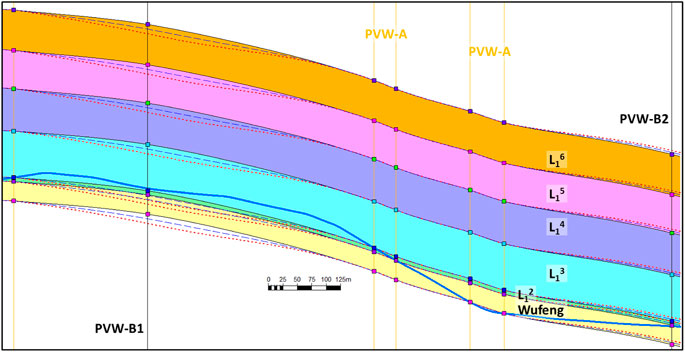
FIGURE 13. The effect of confidential constant on the 3D structural model of shale reservoirs using the cross section along the well JY-b. The black solid lines, the blue dash lines, and the red dot lines represent the structural model using the confidential constant of 95, 85, and 75%.

In order to estimate these process-associated uncertainties, it is necessary to construct multiple 3D structural models using different values of the initial thickness (either a constant value or a contour map), dip angle change threshold, thickness change threshold, and confidential constant and compare their differences. Except the confidential constant, the other three parameters work together to determine the shale layer TVTs. Compared to the dip angle change threshold and thickness change threshold, the initial thickness can be estimated from formation tops in vertical wells, depositional environments, and geologic knowledge of the study area. Meanwhile, the iterative process is designed to update the initial thickness based on the dip angle and thickness change threshold. Therefore, the initial thickness usually has a relatively smaller effect on the 3D structural model. Instead of providing multiple different initial thicknesses, it is more feasible to focus on the effect of dip angle change and thickness change threshold. There are rare data to estimate the confidential constant, and it would be good to test three to five values.

Conclusion

The existence of a large number of horizontal wells in the core area of shale oil and gas plays makes its 3D structural modeling distinct from conventional reservoirs with mainly vertical wells. To construct a high-quality 3D structural model for shale oil and gas fields, it is critical to effectively use the data in horizontal wells. The uncoupled formation tops are the main reason for the abnormal thickness in the constructed 3D structural models. Our method is to add PVW-As at all formation tops in horizontal wells and infer the formation tops in all PVW-As based on the thickness of shale layers. As one key component of our method, an iterative process was developed to estimate the shale thickness using the uncoupled formation tops in horizontal wells by balancing the thickness change and dip angle change threshold. Meanwhile, we introduced a new data type, landing formation, in horizontal wells as a soft constraint for the 3D structural modeling. The landing formation data are mainly used to 1) detect whether the horizontal wells land in the correct formation in the constructed 3D structural models and 2) provide the necessary information for adding PVW-Bs if any incorrect landing formation in the 3D structural model is detected.

By adding PVW-As to convert the uncoupled formation tops to coupled formation tops, estimating shale thickness by balancing the dip angle change and the thickness change, detecting errors in the constructed 3D structural model, and adding PVW-Bs to fix these error, we are able to maximize the use of the structural-associated data in horizontal wells to optimize the quality of 3D structural modes of shale reservoirs. The data from the Jiaoshiba area in the eastern Sichuan Basin were utilized to successfully construct two 3D structural models of the Wufeng–Longmaxi Shale reservoir at the well pad scale and the field scale, respectively. Besides, we analyzed the uncertainty within the 3D structural model using horizontal well data, including the uncertainty level, the uncertainty source, and the method to reduce these uncertainties for different data types. This research, by summarizing the special features of formation tops in horizontal wells and the main issues in 3D structural modeling using horizontal well data, developed a method to maximize the data in horizontal wells to optimize the quality of 3D structural models of shale reservoirs. It should be helpful for geologists and engineers to improve their 3D structural model of shale reservoirs for property modeling, hydraulic fracturing simulation, well design, etc.

Data Availability Statement

The raw data supporting the conclusions of this article will be made available by the authors, without undue reservation.

Author Contributions

ZS devised the project and wrote a significant part of the study. GW provided the main conceptual ideas and wrote the main part of the manuscript. YL contributed to developing the method, making some of the figures, and analyzing the data. CW, YC, and XZ helped with the manuscript, the figures, and data analysis. All authors contributed to the article and approved the submitted version.

Conflict of Interest

Authors ZS, CW, YC and XZ were employed by the company Sinopec Jianghan Oilfield Company.

The authors declare that this study received funding from the Research Institute of Exploration and Development, SINOPEC Jianghan Oilfield Company. The funder had the following involvement in the study: study design, data collection and analysis, decision to publish, and preparation of the manuscript.

The handling editor is currently organizing a Research Topic with one of the authors GW.

Publisher’s Note

All claims expressed in this article are solely those of the authors and do not necessarily represent those of their affiliated organizations, or those of the publisher, the editors and the reviewers. Any product that may be evaluated in this article, or claim that may be made by its manufacturer, is not guaranteed or endorsed by the publisher.

Acknowledgments

Special thanks to the Research Institute of Exploration and Development, SINOPEC Jianghan Oilfield Company, for providing the necessary data in the Jiaoshiba area, eastern Sichuan Basin for this research.

Supplementary Material

The Supplementary Material for this article can be found online at: https://www.frontiersin.org/articles/10.3389/feart.2021.695502/full#supplementary-material

References

Carter, K. M., Harper, J. A., Schmid, K. W., and Kostelnik, J. (2011). Unconventional Natural Gas Resources in Pennsylvania: The Backstory of the Modern Marcellus Shale Play. Environ. Geosci. 18 (4), 217–257. doi:10.1306/eg.09281111008
Donahoe, T., and Gao, D. (2016). Application of 3D Seismic Attribute Analysis to Structure Interpretation and Hydrocarbon Exploration Southwest Pennsylvania, Central Appalachian Basin: A Case Study. Interpretation 4 (3), T291–T302. doi:10.1190/INT-2015-0080.1
EIA (2019). International Energy Outlook 2019 With Projections to 2050. Available at: https://www.eia.gov/ieo. (Accessed August 10, 2020).
Fomel, S., and Landa, E. (2014). Structural Uncertainty of Time-Migrated Seismic Images. J. Appl. Geophys. 101, 27–30. doi:10.1016/j.jappgeo.2013.11.010
Griffiths, R., Morris, C., Ito, K., Rasmus, J., and Maggs, D. (2012). Formation Evaluation in High Angle and Horizontal wells – A New and Practical Workflow. Paper FF presented at SPWLA 53rd Annual Logging Symposium. Cartagena, Colombia. June 16-20, 2012.
IEA (2019). World Energy Outlook 2019. Available at: https://www.iea.org/reports/world-energy-outlook-2019. (Accessed August 10, 2020).
Jarvie, D. M., Hill, R. J., Ruble, T. E., and Pollastro, R. M. (2007). Unconventional Shale-Gas Systems: The Mississippian Barnett Shale of north-central Texas as One Model for Thermogenic Shale-Gas Assessment. Bulletin 91 (4), 475–499. doi:10.1306/12190606068
Krajnovich, A., Zhou, W., and Gutierrez, M. (2020). Uncertainty Assessment for 3D Geologic Modeling of Fault Zones Based on Geologic Inputs and Prior Knowledge. Solid Earth 11, 1457–1474. doi:10.5194/se-11-1457-2020
Lelliott, M. R., Cave, M. R., and Wealthall, G. P. (2009). A Structured Approach to the Measurement of Uncertainty in 3D Geological Models. Q. J. Eng. Geology Hydrogeology 42, 95–105. doi:10.1144/1470-9236/07-081
Liang, D., Hua, W., Liu, X., Zhao, Y., and Liu, Z. (2021). Uncertainty Assessment of a 3D Geological Model by Integrating Data Errors, Spatial Variations and Cognition Bias. Earth Sci. Inform. 14, 161–178. doi:10.1007/s12145-020-00548-4
Liu, X. (2018). Borehole Trajectory Uncertainty and its Characterization. Pet. Exploration Dev. 46 (2), 407–412. doi:10.1016/S1876-3804(19)60021-2
Long, S., Zhang, Y., Li, J., Sun, Z., Shang, X., and Dai, C. (2019). Comprehensive Geological Modeling Technology for Shale Gas Reservoirs. Nat. Gas Industry 3, 47–55. doi:10.3787/j.issn.1000-0976.2019.03.006 in Chinese.
Maggs, D., Lattuada, S., Griffiths, R., Mele, M., and Valdisturlo, A. (2014). Petrophysics in High Angle and Horizontal wells. Proc. GEO ExPro 11 (1), 60–62.
Passey, Q. R., Yin, H., Rendero, C. M., and Fitz, D. E. (2005). Overview of High-Angle and Horizontal Well Formation Evaluation: Issues, Learning and Future Directions. Paper A, SPWLA 46th Annual Logging Symposium, New Orleans, Louisiana, June 16-20, 2012.
Pinto, V. R., Abreu, C. E. B. d. S., Monteiro, R. C., Rosseto, J., and Leahey, G. M. (2017). Seismic Uncertainty Estimation in Reservoir Structural Modelling. First Break 35 (10), 51–54. doi:10.3997/1365-2397.35.10.90243
Qiao, H., Jia, A., and Wei, Y. (2018). Geological Information Analysis of Horizontal wells and 3D Modeling of Shale Gas Reservoirs. J. Southwest Pet. Univ. (Science Tech. Edition) 40 (1), 78–88. in Chinese. doi:10.11885/j.issn.1674-5086.2017.05.10.04
Shahkarami, A., and Wang, G. (2017). Horizontal Well Spacing and Hydraulic Fracturing Design Optimization: a Case Study on Utica-Point Pleasant Shale Play. J Sustain. Energy Engng 5 (2), 148–162. doi:10.7569/jsee.2017.629508
Shtuka, A., Hadziavdic, V., and Sandjivy, L. (2018). Dealing with Uncertainty on Horizontal Well Trajectory when Targeting New Infill Drilling: The Brage Field Case Study. 80th EAGE Conference and Exhibition. Copenhagen, Denmark: June 11-14, 2865–2869. doi:10.3997/2214-4609.201801236
Shu, H., Wang, L., Yin, K., Li, Q., Zhang, Z., and Luo, Y. (2020). Geological Modeling of Shale Gas Reservoir during the Implementation Process of Geology-Engineering Integration. China Pet. Exploration 25 (2), 84–95. in Chinese. doi:10.3969/j.issn.1672-7703.2020.02.009
Stein, M. L. (1999). Interpolation of Spatial Data: Some Theory for Kriging (Springer Series in Statistics). Springer. doi:10.1007/978-1-4612-1494-6
Wang, G., and Carr, T. R. (2013). Organic-rich Marcellus Shale Lithofacies Modeling and Distribution Pattern Analysis in the Appalachian basin. Bulletin 97 (12), 2173–2205. doi:10.1306/05141312135
Wang, G., Long, S., Ju, Y., Huang, C., and Peng, Y. (2018a). Application of Horizontal wells in Three-Dimensional Shale Reservoir Modeling: A Case Study of Longmaxi-Wufeng Shale in Fuling Gas Field, Sichuan Basin. Bulletin 102 (11), 2333–2354. doi:10.1306/0924191908110.1306/05111817144
Wang, G., Long, S., Ju, Y., Huang, C., and Peng, Y. (2018b). Issues of Horizontal Well Log Interpretation: An Example Longmaxi-Wufeng Shale in Fuling Gas Field of Eastern Sichuan Basin. Joint Eastern Section AAPG/SPE Conference. Pittsburgh, PA: October 2018.
Wang, Z. (2015). Breakthrough of Fuling Shale Gas Exploration and Development and its Inspiration. Oil Gas Geology 36 (1), 1–6. doi:10.11743/ogg20150101 in Chinese.
Wellmann, J. F., Lindsay, M., Poh, J., and Jessell, M. (2014). Validating 3-D Structural Models with Geological Knowledge for Improved Uncertainty Evaluations. Energ. Proced. 59, 374–381. doi:10.1016/j.egypro.2014.10.391
Keywords: shale reservoir, horizontal well, 3D structural modeling, pseudo vertical well, landing formation
Citation: Shu Z, Wang G, Luo Y, Wang C, Chen Y and Zou X (2021) Shale Reservoir 3D Structural Modeling Using Horizontal Well Data: Main Issues and an Improved Method. Front. Earth Sci. 9:695502. doi: 10.3389/feart.2021.695502
Received: 15 April 2021; Accepted: 05 July 2021;
Published: 12 August 2021.
Edited by:
Min Wang, China University of Petroleum (Huadong), ChinaReviewed by:
Charles Makoundi, University of Tasmania, AustraliaLiaosha Song, California State University, Bakersfield, United States
Copyright © 2021 Shu, Wang, Luo, Wang, Chen and Zou. This is an open-access article distributed under the terms of the Creative Commons Attribution License (CC BY). The use, distribution or reproduction in other forums is permitted, provided the original author(s) and the copyright owner(s) are credited and that the original publication in this journal is cited, in accordance with accepted academic practice. No use, distribution or reproduction is permitted which does not comply with these terms.
*Correspondence: Guochang Wang, gwang@francis.edu