Climate Change Impact on the Offshore Wind Energy Over the North Sea and the Irish Sea

Introduction

The impact of climate change on the environment and human activities is one of the biggest concerns for the international community and led to the institution of the Intergovernmental Panel on Climate Change (IPCC) in 1988. IPCC Special Report on Global Warming of 1.5°C (Masson-Delmotte et al., 2018) highlighted the importance of containing the temperature increase below 1.5° over the preindustrial levels to reduce the risk of extreme events (droughts, heavy precipitations). This objective can be reached through a drastic reduction of emissions, among other strategies. Electricity and heat generation sectors accounted for the largest share of global greenhouse gas (GHG) emissions (EPA, 2019), principal responsible for global warming (Stott et al., 2000; Meehl et al., 2004; Stone et al., 2007), while during the third quarter of 2021 electricity and heat generation sectors accounted for the second-largest share of GHG emissions in Europe (https://ec.europa.eu/eurostat). Hence, a firm effort is currently aimed at harvesting renewable energy sources. Wind plays a leading role in Europe with 236 GW of cumulative installed capacity in 2021 covering 15% of Europe’s electricity demand in the same year. Offshore capacity has increased its importance in recent years, as it grew from 1% of the total installed wind power in 2008 to 19% in 2021 (Komusanac et al., 2022). The European Commission expects a further increase in the coming decades, which will bring the installed offshore capacity from the current 12 GW up to 300 GW in 2050 (European Commission, 2020). An accurate description of the environmental conditions is required to facilitate this progressive shift to offshore areas, generally characterized by more intense and uniform wind resources (Esteban et al., 2011). Climate change, in turn, may indeed influence the wind resources in terms of spatial distribution and temporal variability (Pryor et al., 2005). The model proposed by Hdidouan and Staffell (2017) shows that these variations have a relevant impact on the Levelized Cost of Energy (LCoE) evaluation. The process from the early concept design to the decommissioning of an offshore wind farm can last 40 years, without considering repowering strategies that represent a valuable alternative to decommissioning due to cost optimization and sustainability (Hou et al., 2017). Hence it appears clear that changes in the wind resource in the upcoming 50–70 years can impact wind farms currently in operation (Carvalho et al., 2017).

North Sea is particularly strategic for the wind energy industry, representing the vast majority of the total European installed power (Ramirez et al., 2020). The effects of variations in large-scale circulation are expected to modify the frequency of climate extremes in North Europe (Scaife et al., 2008). Zheng et al. (2019) and Carvalho et al. (2017) analyzed projections of future global offshore wind energy resources using data from the Coupled Model Intercomparison Project (CMIP) under various RCP scenarios, finding an overall reduction in the wind power density over the North and the Irish Sea. McInnes et al. (2011) found an overall increase of the 99thi percentile daily wind speed up to 5% in the North Sea, following an ensemble approach based on CMIP3 simulations downscaled through RCA4. Moemken et al. (2018) observed an increase in the time in which the wind speed is below the cut-in threshold and a consequent reduction of the operational intervals for typical wind turbines. The distribution of projected changes between model simluations varies considerably, both in sign and in strength, as also found by Meier et al. (2011) and De Winter et al. (2013). Signs discrepancies between simulations are particularly evident in the southern North Sea region, to the point that Sterl et al. (2015) suggest that changes found in the literature are not statistically significant. However, these results rely on the outcomes from Atmospheric Ocean General Circulation Models (AO-GCMs) characterized by a coarse spatial resolution, unable to solve meso-scale circulation features over the analyzed seas. In order to support stakeholders during the decision-making process, there is a need for regional climate information on the impact that climate change may have on the offshore wind industry (Murcia et al., 2015). Few studies so far have investigated the climate change impact on the offshore wind energy sector at a local scale, mainly due to the lack of information about real turbines power curves, which are generally substituted by idealized power curves (Weber et al., 2018; Ohba, 2019). Doddy Clarke et al. (2022) analyzed more than 20 onshore and offshore wind farms in Ireland, finding a decrease of up to 2% in the wind energy potential.

This study describes an evaluation of the impact of climate change in the offshore wind sector over the North Sea and the Irish Sea regions (Figure 1) employing an ensemble of regional climate model (RCM) simulations forced by CMIP5 global models. We conduct a weather type analysis both as a basis for assessing the skill of the RCM simulations and for providing the geographical distribution of future changes. After evaluating projected changes within the marine region with a high spatial resolution (∼10 km), we calculate several indicators for seven offshore wind farms. The model simulations considered are affected by systematic deviations (bias) from their reference period, and hence data need calibration to be suitable for climate change impact study. To this aim, we apply the empirical quantile mapping technique to the modeled wind time series coming from RCM simulations. We employ in-situ records to validate historical information from the ERA5 reanalysis and then use the validated ERA5 data to support the bias correction procedure of the RCMs. We focus on long-term climate changes, comparing a reference historical period (1985-2004) with the future time slice 2081-2100 under the RCP8.5 GHG emissions scenario. The RCP8.5 scenario represents the emission trajectory associated with the most intense radiative forcing (8.5 W/m2) and hence the highest GHG levels among the concentration pathways individuated by the IPCC. Although a more near time window (i.e. mid-century) could be convenient for specific engineering applications and policies redaction, we focus on the end of the present century, which yields the maximum robustness for changes (Moemken et al., 2018) and allows to tackle the climate change issue in a broader perspective. The paper is organized as follows. In Data Source Section, datasets used for the work are described. Methods Section provides information about methods applied for weather type (WT) classification, skill assessment of the RCM simulations, bias correction, and the definitions of wind energy indicators. Results are presented in Result and Discussion Section, and conclusions are given in Conclusion Section.

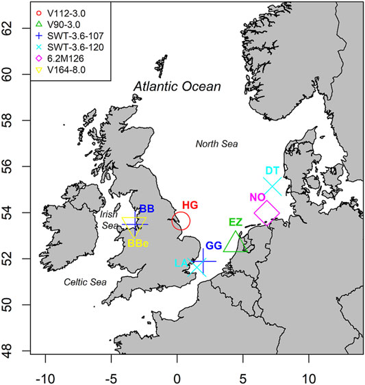
FIGURE 1. Study area and map of the analyzed offshore wind farms. Legend indicates the turbine models for each wind farm.

Data Source

Offshore In-Situ Records

In-situ records provide valuable information for offshore wind farms, although they may be affected by micro-scale processes, such as the wake of turbines. In addition, data from these records contain gaps and are usually short for a robust long-term climate characterization. The records from seven currently operating offshore wind farms are selected and used to validate the historical information from the ERA5 reanalysis. The location of the records is indicated in Figure 1, as well as the turbine model employed in each offshore wind farm.

Heterogeneous conditions (e.g. distance to the coast and type of installed turbine) affecting the energy production, are therefore considered. Time series of wind speed and direction have been gathered from Marine Data Exchange (www.marinedataexchange.co.uk), FINO (www.fino1.de), and Nordzee-wind (Brand et al., 2012) databases. Their available time period and other characteristics are summarized in Table 1.

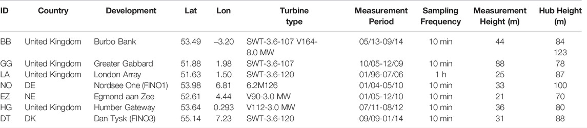
TABLE 1. List of the in-situ observations used and characteristics of the wind speed time series at the analyzed offshore wind farms.

Table 1 data were collected mainly before park commissioning and hence are not affected by the wakes of the wind turbines. Egmond aan Zee and Dan Tysk parks constitute the only exceptions in this sense, but the analysis of wind rose distributions and probability density functions show that the effects of wakes did not affect the quality of measurements. We conduct additional quality control to eliminate outliers, and then we operate an hourly average on the 10-min original values to make them directly comparable with the ERA5 reanalysis hourly data.

Atmospheric Reanalysis Data

The recent ERA5 reanalysis product of the European Centre for Medium-Range Weather Forecasts (ECMWF) is adopted here as a quasi-real historical dataset due to the unavailability of sufficiently long and homogenous observational time series covering a region as broad as the target of this study. The ERA5 (Hersbach et al., 2020) HRES (high resolution) atmospheric data are provided on a 31 km horizontal grid with hourly time resolution. Reanalysis data have been preprocessed in order to serve a double purpose. Firstly, the spatial wind at 10 m height (zonal u and meridional v wind components) and sea level pressure (slp) hourly fields are converted into daily mean values for the period 1985-2004 in order to be used for the classification of atmospheric circulation patterns. Then, we employ the historical information provided by ERA5 as reference datasets for the historical conditions provided by regional climate simulations.

ERA5 capabilities have already been assessed in several works. In terms of wind power modeling, ERA5 performs better than other reanalyses such as the MERRA-2 dataset (Olauson, 2018; Jourdier, 2020). Sharmar and Markina (2020) concluded the same after analyzing global wind wave hindcasts, while Rivas and Stoffelen (2019) conducted a global comparison with ASCAT observations which highlighted a 20% bias reduction compared to ERA-INTERIM (Dee et al., 2011). The hourly wind speed time series provided by ERA5 are here validated through a comparison with the available in-situ records. To this aim, we interpolate the wind time series at the farm height location following the power relationship shown in Eq. 1 to scale the 10 m values (w₁₀) up to the measurement height (h_m) specific to each park, as listed in the last column of Table 1.

The exponent α depends on multiple factors such as elevation, time of day, and temperature. Under neutral conditions and with flat terrain, α is equal to 0.14 (Schlichting 1968), which is also the value suggested by the International Electrotechnical Commission (IEC, 2019) for offshore locations. In conformity with several previous studies (e.g. Hueging et al., 2013; Moemken et al., 2018), we adopt the value α = 0.14 for the present study.

Figure 2 provides the comparison between ERA5 wind speed data and instrumental measurements at the seven wind farm sites. The scatter plots show the pairs of hourly data values (colored according to their probability of occurrence) and the percentiles of the distribution. The quality of the ERA5 wind data is confirmed by the small values assumed by root mean square error (RMSE), which is always lower than 2 m/s. Lowest value is shown at Dan Tysk (RMSE = 1.1886 m/s), while the highest is found in correspondence of London Array (RMSE = 1.7313 m/s). We observe some slight underestimation in the farms near the United Kingdom coast and an overestimation in the farms near the Netherlands, Germany, and Denmark.

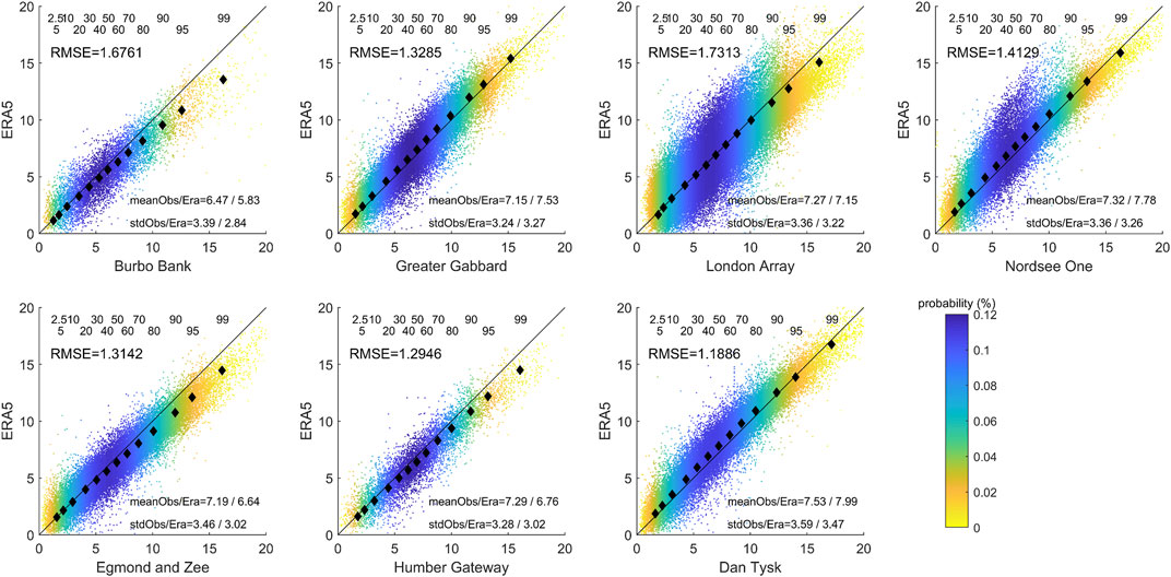
FIGURE 2. Comparison of ERA5 against the in-situ measured data at the seven analyzed offshore parks. Probability scatter diagrams are colored by density of data. Black diamonds are the quantiles, from 2.5 to 99 as indicated on the top of each panel. The difference in the mean and standard deviation as well as the RMSE (m/s) are also indicated.

Climate Models

The fifth IPCC Assessment Report (AR5) is based on the results provided by the Coupled Model Intercomparison Project Phase 5 (CMIP5). The CMIP5 consists of a multi-model approach for assessing AO-GCM capabilities and limitations, providing a freely available dataset designed to advance the knowledge of climate variability and climate change (Taylor et al., 2011). The investigation of the climate change impact through an ensemble approach based on a multi-model analysis provides a more skillful result and reduces the sources of uncertainty (Tebaldi and Knutti, 2007). Assessing the skills of the climate models for a specific region on the basis of how well they reproduce the synoptic climatology provides a more complete evaluation than the mere comparison of statistics against observational sources. Clustering methods are usually applied under this approach. (e.g. Perez et al., 2014; Belleflamme et al., 2013; Lorenzo et al., 2011), with the advantage of reducing climate time variability to a limited set of circulation patterns.

GCMs are the most advanced tools available for simulating physical processes of the global climate system in response to different greenhouse gas concentration emissions. However, they are characterized by a coarse spatial resolution (in the order of the hundreds of km), insufficient to satisfactory project climate conditions at meso-to micro-scales. This problem can be relevant in areas characterized by complex geography elements such as the North Sea and the Irish Sea. Regional Climate Models (RCMs) are employed to overcome this limitation, increasing resolution over a specific region towards a horizontal grid-point spacing of a few tens of km (Laprise, 2008). Progressive developments in the available computer power and storage capacity have allowed setting the standard resolution for regional downscaling at 12 km. The Euro-CORDEX initiative (Coordinated Regional Climate Downscaling Experiment) provides higher-resolution regional climate information that is available directly from contemporary global climate models in a European domain (Jacob et al., 2014). Euro-CORDEX aims to assess the performance of downscaling models, designing a set of coherent experiments for the production of climate projections to be used in impact and adaptation studies (Giorgi et al., 2009).

We select those Euro-CORDEX simulations that provide continuous wind speed and atmospheric sea level pressure data with high spatial (0.11°) and temporal resolution (6-hourly) for the RCP8.5 scenario during the 20-years future time slice 2081-2100 and with the availability of the same experiment during a historical reference period (1985-2004). The resulting simulations are listed in Table 2. CanESM2 and MIROC5 are downscaled through COSMO-CCLM4-8-17 (Rockel et al., 2008), while CNRM-CM5, EC-EARTH, HadGem2-ES, IPSL-CM5A and MPI-ESM-LR are downscaled through RCA4 (Kupiainen et al., 2011). From now on, we refer to a simulation through the name of the regionalization scheme followed by the parent GCM model between brackets (e.g., CCLM(CanESM2) and RCA4(CNRM-CM5)).

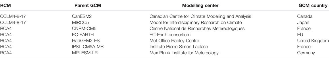
TABLE 2. List of the analyzed RCM simulations and their downscaled GCMs from CMIP5.

Methods

The methodological approach followed can be ideally split into two different streams of analysis. In the first one, we operate at a meso-scale perspective to classify the synoptic patterns of the target area and successively make use of this classification for assessing the performance of the climate model simulations. Then we move up to the detail study, focusing on seven operating offshore windfarms: regional climate data are bias-corrected as described within Bias Correction Section and successively employed to calculate relevant wind energy indicators.

Classification of Atmospheric Circulation Patterns

We apply a non-hierarchical clustering approach to obtain atmospheric circulation patterns in the target region. These patterns are then used to explain the future changes in offshore wind energy that regional climate projections predict by analyzing variations in their frequency of occurrence.

The clustering method classifies the meteorological circulation systems over the marine surface of the studied area into weather types (WT), in such a way that each WT represents an atmospheric circulation pattern. In this approach, a principal component analysis (PCA) is first applied to the selected variables to reduce the data dimensionality while conserving maximum data variance. The result is a new set of variables (principal components, PCs) that are linearly dependent on the original ones and uncorrelated between each other. The classification algorithm is applied to them, simplifying the classification problem into an eigenvalue/eigenvector problem (Jolliffe and Cadima, 2016). To this aim, the maximum-dissimilarity algorithm (MDA) is employed to initiate the clustering process following Camus et al. (2011), which guarantees a stable classification and the most representative initial subset. Finally, we use the K-means algorithm (KMA), which is designed to partition two-way, two-mode data into K classes (Steinley, 2006). This algorithm allows individuating a set of centroids, each of them representative of a group of data formed by the vectors in the database for which the corresponding centroid is the nearest one (Hastie et al., 2001).

The climate of a region can be classified according to several combinations of atmospheric variables, and the choice of the variables to consider when applying the clustering technique depends on the purpose of the system itself (Lee, 2014; Tveito et al., 2016). Siegert et al. (2017) and Cheng et al. (2010) consider a set of six atmospheric variables (sea level pressure, total cloud coverage, air temperature, dew point temperature, eastward and northward wind components), while Camus et al. (2014) focus on pressure data, assuming sea level pressure and squared sea level pressure gradients as predictand for the classification. We explore the sensitivity of the classification technique to different combinations of atmospheric variables and spatial and temporal resolution. As we are primarily interested in describing the wind fields over the study domain, we combine the commonly used sea level pressure (slp) fields with zonal and meridional wind components (u10, v10). Land grid points are excluded in order to focus on the marine surface.

Before PCA processing, anomalies of the selected variables (slp, u10, v10) are calculated from the ERA5 database for the period 1985-2004 and standardized by dividing the difference between actual (V(x,t)) and mean ($\overline{V\left(x\right)}$) value of the generic variable V in the node x by the standard deviation std(V(x)).

The principal components (PCs) obtained from the PCA are then sorted in increasing order of explained variance, and we keep only the PCs that explain 95% of the variance to reduce the problem dimensionality (Perez et al., 2015). In this study, the first eight modes explain 95% of the variance, and the clustering algorithm is hence applied to them. After a sensitivity analysis of the number of WTs of 25, 36, 64 and 100, N = 100 WTs are selected. The selection of 100 clusters arises from a balance between the necessity of obtaining a classification that identifies extreme WTs, and that all groups have sufficient data representation (the obtained WTs comprise 77 daily data per group on average).

The WT classification is visualized in a 10 × 10 lattice for the slp (Figure 3) and wind speed magnitude at 10 m height w₁₀ (Figure 4). For each identified WT, the centroid obtained during the clustering process is substituted by the actual synoptic situation most similar to it. Such a situation is individuated by calculating the Euclidean distance between the points representing all the instants from the historical series belonging to a group and the correspondent group centroid, considering the values assumed by the normalized variables in the point as the point coordinates. The lower-right and upper-left corners of Figure 3 represent situations dominated by low-pressure systems located in the northwestern area of the studied region. They are coupled with intense wind speed (daily mean up to 19 m/s, rotating counterclockwise around depressions generated by cyclonic storms) visible in the same corners of Figure 4. Situations characterized by less intense pressure gradients are displayed in the central part of the lattice and present significantly lower wind speeds.

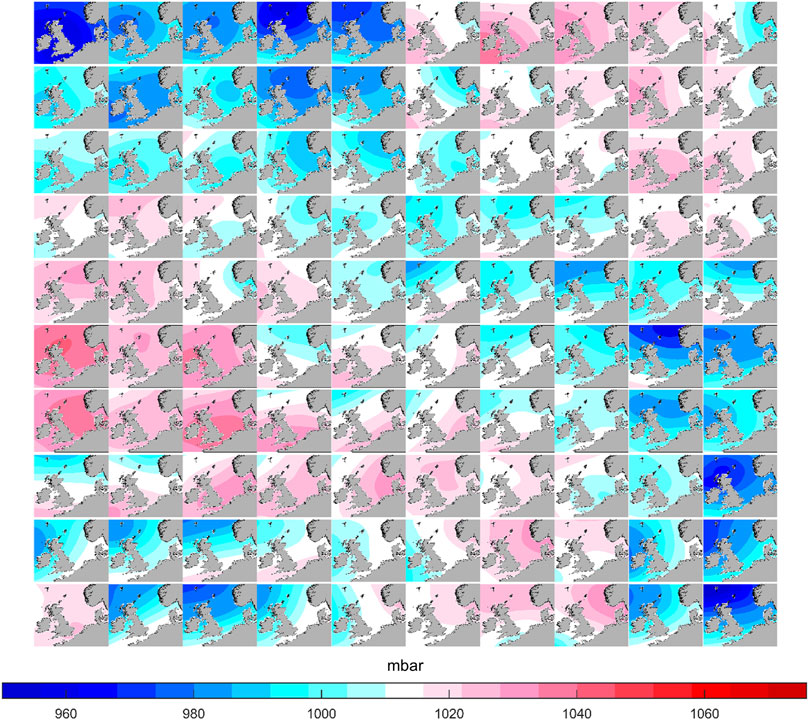
FIGURE 3. The sea level atmospheric pressure fields associated with the weather types, derived from ERA5. Darker blue colors indicate intense low-pressure systems, dominated by a depression generally located in the northwestern area of the studied region. Deep red colors indicate situations of high pressure systems (i.e. anticyclones). Central panels of the lattice show weather types with less intense pressure gradients.

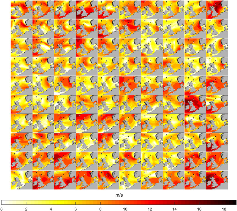
FIGURE 4. The offshore wind speed fields at 10 m height for the 100 weather types, derived from ERA5.

The estimation of the frequency of occurrence of the 100 WTs is used as a benchmark for assessing the skills of RCM simulations and for the analysis of future climate change variations. Figure 5A shows the frequency of occurrence for the ERA5 dataset during the period 1985–2004 calculated by summing up the number of daily situations contained within each of the 100 groups. A similar procedure is repeated considering only the number of occurrences in winter (DJF) and summer (JJA) for each of the individuated WTs (Figures 5B,C, respectively).

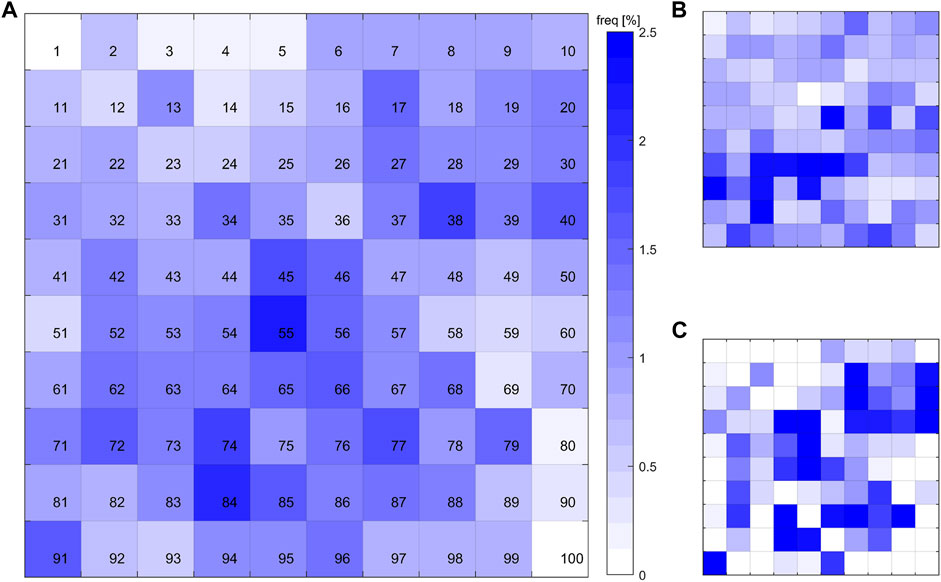
FIGURE 5. Annual (A) winter (B) and summer (C) rate probability occurrence of the 100 weather types (Figures 3, 4 show the atmospheric circulation patterns for each weather type).

The most frequent pattern, represented by WT55 (Figure 6A), describes a situation characterized by a meridional pressure gradient with low pressure located off Far Øer islands, wind speed up to 12 m/s in the northwestern portion of the domain and sensibly lower in the area where the analyzed wind farms are located (except for DT). In summer, WT84 describes the most frequent situation with southeastward pressure gradient and generally lower wind directed towards NE, though we note that all the analyzed offshore plants (with the exclusion of GG and LA) are invested by wind between 6 and 10 m/s, resulting in favorable conditions for energy extraction. The most usual situation in winter is depicted in WT65 (Figure 6B). It is characterized by winds above 10 m/s within the central and northern part of the domain, resulting in good conditions for British plants, while the continental coast of Europe is interested by significantly lower winds. These situations, which are predominant in terms of total occurrences, are characterized by a dualism between high and low pressure systems that originates a definite gradient. WTs dominated by a depression (WT4, Figure 6C) and an anticyclone (WT53, Figure 6D) are less frequent in the studied region. WT4 describes intense winds with daily mean speed up to 19 m/s over the Irish Sea and the British Channel. Such a high value of the daily mean corresponds to survival rather than operational conditions for wind farms, considering that the cut-off speed is around 25-30 m/s depending on the turbine installed. Conversely, WT53 represents a situation in which most of the analyzed wind farms are affected by winds below the cut-in threshold.

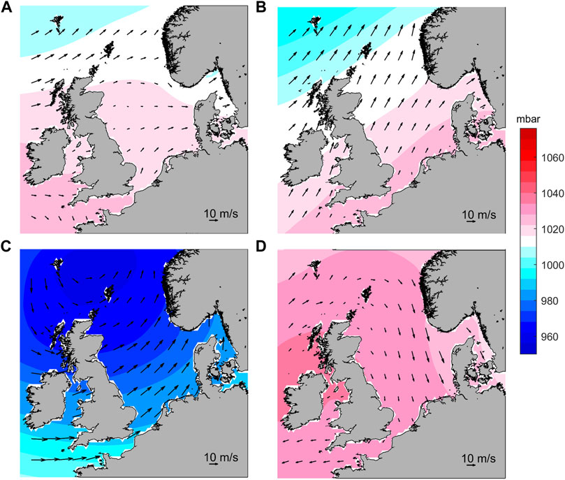
FIGURE 6. Sea level atmospheric pressure and surface wind speed fields of WT55 (A), WT65 (B), WT4 (C), and WT53 (D). WT55 (A) and WT65 (B) represent the most frequent pattern at annual and winter scale, respectively. WT4 (C) and WT53 (D) show cyclonic and anticyclonic situations, respectively.

Performance of the Climate Model Simulations

The WT classification obtained from the historical information of the ERA5 data is used for assessing the performance of the RCM simulations during the reference period (1985-2004). First, simulations are classified by comparing the frequency of occurrence of each WT with the one provided by ERA5 data (shown in Figure 5A). Then, we ensemble the frequency of occurrence of each WT from the seven simulations and compare it with the correspondent frequency from the ERA5 data. Finally, we assess the performance of the RCM simulations in reproducing the interannual variability of the ERA5 reference dataset.

In order to obtain the frequency of occurrence of the 100 WTs for each RCM, the slp, u10, and v10 for each climate simulation are translated to the PCA dimension retrieved from the ERA5 data. Each daily situation is associated with one of the 100 WTs previously individuated from the ERA5 dataset, and the frequency of occurrence of the WTs for each RCM simulation is then computed for the historical period (1985-2004), summing up the number of daily situations contained within each of the 100 groups. The same procedure is then repeated for the period 2081-2100, allowing the investigation of the future variations in the frequency of occurrence of a specific WT due to climate change.

Statistical indexes to compare the difference in the frequency of the WTs from each RCM historical simulation against the frequency of the ERA5 data are estimated in order to quantify the performance of the RCMs (Perez et al., 2014). The scatter index SI and relative entropy RE are calculated from the knowledge of the frequency of occurrence of each group, where p_i is the frequency of occurrence of ith WT from ERA5, p_i’ refers to the frequency of occurrence of the ith WT from an individual RCM simulation, and N is the number of WTs (100).

The RE index, in particular, gears more the WTs characterized by low probability of occurrence (i.e. unusual synoptic conditions).

We also analyze frequency discrepancy (FD_i) between the occurrence of the ith WT from ERA5 (p_i) and the ensemble mean of the frequencies provided by the RCM simulations (p’_i-ENS) through the following formulation.

A criterion to individuate consistency is applied whenever a calculation involves the ensemble of simulations. Following Perez et al. (2014), we identify with black dots those WTs and grid points in which at least 80% of the simulations agree in the sign of the variation.

In order to measure the skill of the climate simulations in the reproduction of interannual variability, the standard deviation of the scatter index stdSI, is also estimated.

Bias Correction

The bias correction process consists of scaling climate model outputs to reduce their systematic errors with the aim to improve their fitting to observations (Soriano et al., 2019). Several bias correction methods (e.g. Déqué 2007; Brands et al., 2011; Tabor and Williams 2011) developed over recent years focused on increasing the quality of climate projections and making them suitable for a proper estimation of indicators in impact studies. The correction procedure is required for the detailed impact assessment study that we conduce at the offshore wind parks (Ahmed et al., 2013).

The ERA5 reanalysis database has proven its good quality to represent wind conditions over the selected offshore wind farms. The validation described for the seven wind farms at the measurement height (Figure 2) indicates modest discrepancies with respect to in-situ records when representing the wind distribution. Therefore, considering that the in-situ records are short and do not cover a common period of enough length, we choose the ERA5 database to undertake a bias correction of the climate model simulations at the seven wind farm locations.

Figure 7 shows a comparison of the wind distribution characterizing ERA5 and the RCM simulations at 10 m height. We note that the RCM simulations tend to overestimate the magnitude of the wind speed for high quantiles. The only exception is represented by the Egmond and Zee wind farm. Most of the analyzed RCM simulations underestimate ERA5 quantiles at this wind farm.

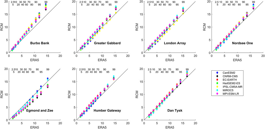
FIGURE 7. Quantile-quantile plots of the comparison between the ERA5 and the seven analyzed regional climate simulations at the seven offshore wind farms. The quantiles range from 2.5th to 99th, as indicated at the top of each panel.

The method designed for bias correction is the Empirical Quantile Mapping (EQM), which maps between simulated and quasi-observed Cumulative Distribution Functions (CDFs). It is implemented following Déqué (2007), thus obtaining a correction function for each of the thirteen selected percentiles (2.5, 5, 10, 20, 30, 40, 50, 60, 70, 80, 90, 95, 99) and linearly interpolating between two percentiles. Outside the range between 2.5 and 99, the extrapolation is set to constant, meaning that the correction function for the 99th percentile is applied to all the above percentiles. ERA5 reanalysis is used to obtain quantile-specific correction coefficients for RCM simulations by comparing climate information at the annual scale for the period 1985-2004. Then, we apply the so-obtained coefficients to both historical and RCP8.5 future time series of the RCM simulations interpolated at the wind farm locations. In this way, we obtain corrected six-hourly time series for the calculation of local wind energy indicators.

Wind Energy Indicators

The analysis of climate change impact on the wind energy industry is provided through a set of relevant impact indicators.

In addition to the often analyzed climatology in the context of climate change impact studies (e.g. mean wind speed and power density), extreme wind speed, annual energy production, capacity factor, and operation time indicators are also introduced in this study. We conduct calculations for each of the seven locations (Burbo Bank is repeated as two different wind turbines are installed there) using bias-corrected wind speed time series of the seven RCM simulations, scaled at the hub height (HH) characteristic of each wind turbine by applying power law (Eq. 1).

The climate change indicators derive from a comparison between future and historical climate conditions, namely hist (from 1985 to 2004) and RCP8.5 (from 2081 to 2100 under the RCP8.5 scenario). They are calculated individually for each RCM simulation, and then their mean value is obtained following the ensemble approach.

Wind Power Density (WPD) represents a quantitative measure of the wind energy flux available at any location and can be used to compare wind resources regardless of the wind turbine size.

w represents the mean wind speed at HH, while the air density $\rho$ is evaluated through the relation proposed by Hennessy to take into account the reduction of the standard value (ρ₀ = 1.225 kg/m³) due to the height effect (Hennessey, 1977).

We investigate not only variations relevant for the energy harvesting (mean values of wind speed and power density) as it is commonly done (Guo et al., 2020) but also extreme wind speed conditions represented by the 99th percentile (w99) wind speed, which play a role in the dimensioning of the turbine support structure.

In addition to the three climatological indicators, we analyze other quantities related to the specific turbine installed at each site. We define the operation time (OT) as the ratio between the number of hours in which the wind speed lays in the interval individuated by cut-in and cut-off (n_cico) wind speed and the total length of the time series (n_tot).

The gross energy yield (AEP_gross) is evaluated through the relation provided by Measnet (2016) guidelines for the evaluation of site-specific wind conditions as follows:

P(w_i) is the power output for each i-esim wind speed bin of unitary width, extrapolated from the power curves provided by manufacturers. H_i is the number of hours in each wind speed bin, calculated as the product between the relative frequency of that bin (obtained through Weibull fit) and the total number of hours in a year n_y.

Finally, the capacity factor (CF), an important indicator of the performance of a generation plant, is calculated by dividing the AEP for the theoretical annual production (product between nameplate capacity P_n and n_y).

Results and Discussion

Performance of Regional Climate Model Simulations

The frequency discrepancies (FD) between the ensemble of the RCM simulations and the ERA5 reanalysis data are given within Figure 8A, in which black dots individuate WTs for which at least 6 simulations out of 7 agree in the sign of the discrepancy. Figure 8B reports the ranking of the seven RCM simulations accordingly to the values assumed by the calculated statistical indexes (SI, RE, and stdSI) for the annual scale only. The values of the statistical indexes for all the temporal scales (annual, winter, and summer) are listed in Table 3. Smaller values of the indexes indicate a higher degree of similarity with ERA5 and hence a better performing simulation (Perez et al., 2014).

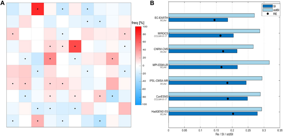
FIGURE 8. Frequency discrepancies (FD) between the ensemble of the regional climate simulations and the ERA5 reference pattern (A). Black dots stand for robustness of FD between model simulations. SI, RE, and stdSI metrics of each of the seven regional climate simulations analyzed (B).

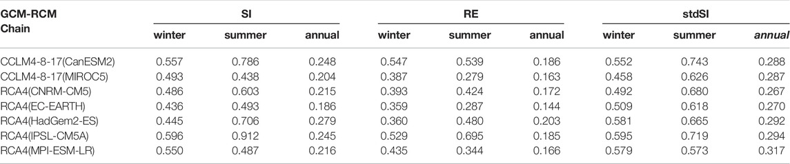
TABLE 3. Performance indexes (SI, RE, stdSI) calculated for each RCM simulation at winter, summer, and annual scale. Best performance in terms of SI and RE is shown by RCA4(EC-EARTH) (annual and winter scale) and CCLM(MIROC5) (summer scale).

Within Figure 8A, we note that the overestimation in the frequency of occurrence of a specific WT is offset by underestimation found in WTs representing similar situations. The same mechanism goes for the opposite. For example, WT36 represents a weak low-pressure system over Far Øer, associated with a daily mean wind speed up to 15 m/s. It describes 43 daily situations of the ERA5 database, while according to the ensemble of RCMs, its frequency of occurrence is higher (+71%, 73 days). This overestimation is explained by a decrease in the frequency of occurrence of similar situations (WT11 and WT79, respectively −12% and −29%), which makes the overall number of days representing this particular synoptic situation comparable between the two datasets (214 days for ERA5, 203 for the ensemble of RCM simulations). Similarly, WT98 is characterized by a pressure gradient increasing towards NE. It represents 60 daily situations of the ERA5 database, while only 41 occurrences (−31%) are found for the ensemble of the RCMs. However, the frequency of occurrence of the similar WT87 is slightly overestimated by the ensemble of the RCMs with respect to ERA5 (116 daily situations against 102), which makes the total number of daily situations associated to this synoptic situation comparable between the two datasets (162 for ERA5 and 157 for the ensemble of the RCMs). Such a compensation mechanism is verified for various groups of WTs representing similar situations and proves the increased ability of the ensemble of the RCM simulations over the individual members in reproducing the historical information from the ERA5 reanalysis.

Moving to the skill assessment of individual model simulations, frequencies obtained from RCA4(EC-EARTH), RCA4(MPI-ESM-LR), RCA4(CNRM-CM5), and CCLM(MIROC5) are generally more similar to the ERA5 reference pattern compared to CCLM(CanESM2), RCA4(IPSL-CM5A), and RCA4(HadGem2-ES). Indeed, they rank in the first four positions of both the annual (Figure 8B) and summer (not shown) time scale. We note the good skill of RCA4(HadGem2-ES) in reproducing winter patterns despite its low performance at the annual and summer scale. The best performing simulation is RCA4(EC-EARTH), which ranks in the first position for both annual and winter timescale, followed by RCA4(CNRM5-CM5) and CCLM(MIROC5) which is found to be the best in reproducing summer patterns. In this sense, no clear preference about which of the two regionalization schemes performs better can be expressed due to the fact that only two regional models have been considered. The difference between the top-four model simulations and the remaining appears evident when considering summer patterns, with the worst-performing simulation (RCA4(IPSL-CM5A-MR)) assuming a SI value approximately double with respect to the best-performing ones (Table 3, column 2).

Although RCA4(EC-EARTH) and CCLM(MIROC5) show a better capacity to reproduce inter-annual variability (they rank in the top three for all the time scales considered), differences between simulations are lower for the stdSI index. This finding oriented our choice of considering all seven simulations for the ensemble mean, supported by the notion that a higher number of models allows a better characterization of the uncertainty. The validity of this choice is ensured through the application of the IQR method for outlier detection, a common procedure in statistical software. We verify that all the values assumed by the indexes lay in the interval between the first quartile minus 1.5 times the interquartile range (IQR) and the third quartile plus 1.5 IQR (except for RCA4(MPI-ESM-LR) in stdSI).

Wind Climate Projections of Future Changes

Besides providing a validation benchmark for the RCM simulations, the WT classification allows us to explain the future evolution of atmospheric circulation patterns. Indeed, the variations in the frequency of occurrence of similar weather types let us estimate the differences in the mean and extreme statistics of the distribution of the wind speed. We calculate the variation in the frequency of the i-esim WT (FV_i) for all the RCM simulations analyzed by comparing the historical (p_{i_hist}) and the projected (p_{i_rcp85}) probability of occurrence.

Figure 9 shows the sign of the ensemble mean of the projected frequency variations, where yellow and light blue squares represent respectively frequency increases and decreases. Black dots individuate WTs characterized by robust changes (for which at least 6 simulations out of 7 agree on the sign of the variation).

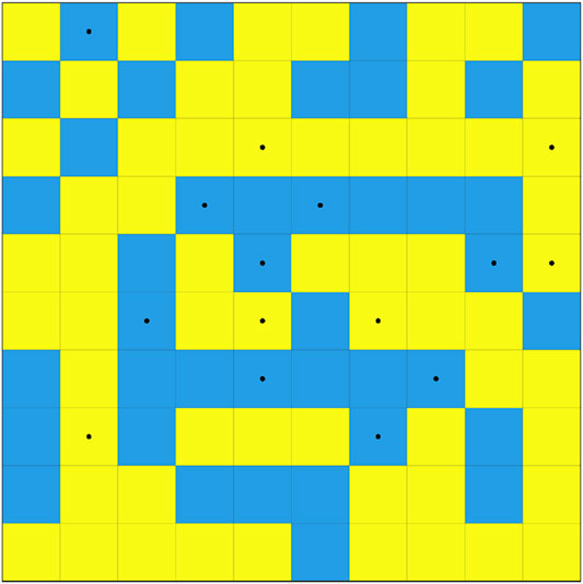
FIGURE 9. Positive (yellow) and negative (blue) frequency variations between the future time slice 2081-2100 under RCP8.5 scenario and historical climate from the ensemble of the regional climate simulations. Black dots stand for change consistency.

We find that WTs representing similar synoptic situations often show a similar pattern of change. For example, situations characterized by intense low-pressure systems located in the NW part of the domain (WT3, WT80, WT90, WT94, WT99, WT100, WT93) are expected to increase in their occurrence by a 10% factor (+31 days in 20 years). On the other hand, situations characterized by less intense pressure gradients (WT36, WT11, WT79, WT64, WT65, WT71) will likely reduce their occurrence in the future.

These modifications at the synoptic scale have a direct impact on mean and extreme climatology. Indeed, the variations in the frequency of occurrence of similar weather types let us estimate the differences in the mean and extreme statistics of the distribution of the wind speed. Figure 10A shows the mean wind speed difference between the future and historical climate. A southeastward gradient appears, with the most intense mean wind speed decrease (−0.6 m/s) in the NW part of the domain and near-zero values off the Danish coasts. A maximum increase of 0.4 m/s is found for the 99th percentile wind speed (Figure 10B) along the continental coast of Europe and in Skagerrak, in accordance with the expected frequency increase of WT3, WT80, WT90, WT93, WT94, WT99, and WT100, which are all characterized by strong winds in those areas. A reduction of the w₉₉ of about 0.5 m/s over the offshore regions of Scotland and Norway is observed. We note that while robustness is guaranteed within the NW part of the domain for the changes in mean wind speed, the extreme wind speed map exhibits consistency off the coasts of Germany, Denmark, Netherlands, and eastern France.

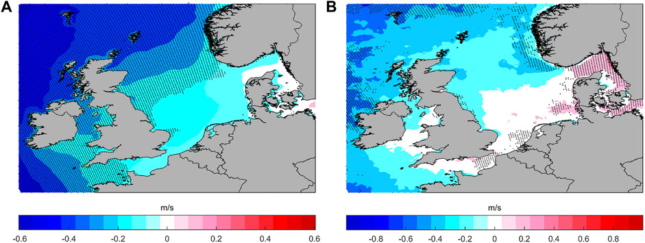
FIGURE 10. Projected variations in mean wind speed (A), 99th percentile wind speed (B) for the period 2081-2100 under RCP8.5 scenario. Black dots stand for results robustness.

Wind Energy Indicators Variations

The results of the calculations described in Wind energy indicators Section are contained within Table 4 for historical and future climate conditions under the RCP8.5 scenario. We evaluate the mean ensemble of the changes in the energy indicators calculated at the hub height as the difference between end-century (2081-2100) and reference historical (1985-2004) period.

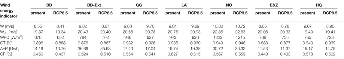
TABLE 4. Climate change energy indicators at the analyzed offshore wind farms (each indicated by its ID as shown in Table 1) for the historical climate (using the 1985-2004 period) and the future time slice (1981-2100) under RCP8.5 scenario: mean wind speed (W), 99th percentile of wind speed (W99), wind power density (WPD), operation time (OT), annual energy production (AEP), and capacity factor (CF).

The analysis of mean wind speed at hub height highlights a slight but robust decrease in the order of 0.1 m/s for all the OWFs considered, more intense for the British plants (biggest decrease for HG). The same spatial distribution characterizes wind power density, which is expected to decrease by a factor up to 4% at HG. Projected variations in the 99th percentile wind speed are positive for all the OWFs located along the English Channel and the coast of continental Europe (with the highest value of 0.3 m/s registered for DT), and almost null for BB and BBext plants. These findings are consistent with the increase in the frequency of WTs dominated by low-pressure systems in the NW part of the domain. The reduction of the operation time (OT), which represents the number of hours in which each turbine operates, is greater at BBext (almost -1%), while it is almost null for NO and DT.

Moving to the indicators more closely related to electric performances of a power plant, from the analysis of the gross energy yield (Figure 11A) it emerges that the BBext plant, equipped with large 8 MW Vestas turbines, is characterized by the biggest production. It is expected to experiment a significant decrease by the end of the century, passing from 36.7 Gwh to 35.7 Gwh (−2.7%), similarly to HG (−2.8%). The remaining plants show a limited decrease in the annual energy production, with reductions between 1 and 2%. The capacity factor (Figure 11B), is directly proportional to the gross energy yield, and consequently, it decreases by the same percentage quantity as the AEP. Higher values are shown in correspondence of DT plant both for historical (70.2%) and for RCP8.5 (69.5%) period, meaning that this plant has a better performance with respect to ones employing larger turbines in terms of the ratio between generated and installed power. We notice however that the confidence intervals showed in Figure 11 indicate a large uncertainty in the projected changes. Nevertheless, the statistical significance of the change in the capacity factor for the BB, BBext, HG and DT wind farms is higher than 65%.

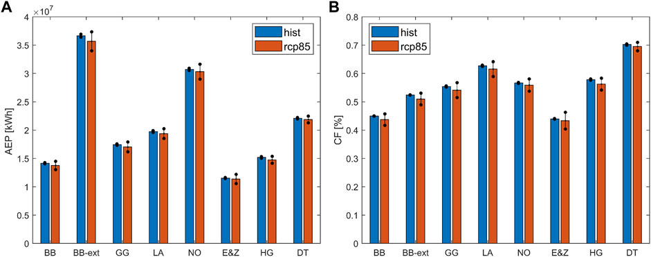
FIGURE 11. Future (orange) and historical (blue) ensemble mean values of Annual Energy Production (A) and Capacity Factor (B) for all the offshore developments analyzed. Black dots indicate the range individuated by the mean value ±1.5 times the standard deviation.

The overall reduction observed for the energy performance indicators is a direct consequence of the observed decrease in the mean wind speed and operation time. The simultaneous increase in extreme events (w₉₉) with consequent shutoff of the generators to avoid damages further contributes to the reduction observed in the energy performance indicators. The increase detected in the w₉₉ suggests that future research may be aimed to understand the projected changes in wind storms.

Conclusion

In this study, we investigate projected changes in the offshore wind resource over the North Sea and the Irish Sea region both at a spatial and local scale by calculating relevant indicators for the wind energy industry. With this aim, a methodology to assess the performance of regional climate model simulations (RCM) in describing synoptic climatology over the target region is applied.

The Weather Type (WT) classification is developed through a data mining approach based on ERA5 reanalysis sea level pressure and directional wind speed fields. The skills of the simulations in reproducing historical climatology is assessed through the calculation of frequency-based statistical indexes (SI, RE, stdSI). The best performing simulation is RCA4(EC-EARTH), which is characterized by the lowest values of both SI and RE at annual and winter scale and ranks in the top three positions for the remaining indexes (SI and RE at summer scale, stdSI), followed by RCA4(CNRM5) and CCLM(MIROC5), which is the best in reproducing summer season patterns. The values of the indexes show low variance for all the simulations analyzed, especially as regards the interannual variability (stdSI). Indeed, the quasi-totality of them lay in the range of the first/third quartile minus/plus 1.5 times IQR. The only exception is represented by RCA4(MPI-ESM-LR) for the stdSI metric. Hence, the choice of considering the seven simulations without disregarding any of them for the ensemble approach appears motivated. A more structured model ensemble including members simulated with several RCMs (we use only simulations from two regional models, i.e., RCA4 and CCLM-4-8-17) is required to analyze the sensitivity of the downscaling scheme. Indeed, Fernández et al. (2019) found that different RCM models driven by the same GCM provide shifts in the projected changes for temperature and precipitation variables for mid-term future slices. They, however, suggest that representative concentration scenarios are the principle uncertainty source in the long term. Accordingly, Toimil et al. (2021) show that the uncertainties related to the description of the future concentration pathways are the main uncertainty contribution for distant future time slices in climate change impact studies. In any case, the GCM-RCM chains used in this study fulfill the institutional democracy criterion that Leduc et al. (2016) propose as a first proxy to obtain an independent subset of simulations.

A comparison between the ensemble of the RCM simulations and ERA5 frequency maps for the historical period suggests a good performance of the climate simulations. The comparison however shows frequency discrepancies between the climate simulation and ERA5 historical data for similar atmospheric circulation patterns. These discrepancies are related to the location of the high/low pressure systems, intensity of gradients between isobars, small regions with specific wind direction and intensity patterns, etc. The analysis of future projections exhibits a tendency towards an increase in the frequency of WTs dominated by low-pressure systems located in the NW part of the domain, characterized by high wind speed in the British Channel and off Norway and Irish coasts. This finding agrees with the projected increase in the proportion of westerly winds found in several authors (Ruosteenoja et al., 2019). Mean wind speed is expected to decrease up to -0.5 m/s off the Atlantic coast of Scotland and Ireland. As WPD has a cubic dependence on mean wind speed, this finding is consistent with the reduction of the mean WPD observed in Zheng et al. (2019) for RCP scenarios 2.5 and 4.6. This evidence would suggest a negative projected trend for the wind resource in this area, regardless of the concentration scenario adopted as forcing for the GCM. Furthermore, we note that in this region the considered simulations show a good agreement, as at least 6 out of 7 agree on the sign of the projected change. On the other hand, changes are not significant in the central part of the domain, as the sign of the modifications varies largely between simulations. This finding is consistent with the conclusions of Carvalho et al. (2017), who applied a Mann-Whitney test with a 5% significance level. A tendency towards an increment of extreme conditions is highlighted along the coast of continental Europe, consistently with the findings of McInnes et al. (2011).

ERA5 dataset is locally validated against in situ observations at seven operating offshore wind farm sites, confirming the conclusions of previous studies (Olauson, 2018; Jourdier, 2020; Sharmar and Markina, 2020) about its quality. We hence employ it for the bias correction of historical and future time series provided by the RCM simulations at the offshore wind farm sites. The corrected time series are then used to evaluate projected variations of impact indicators for the wind energy industry. In accordance with the results of the spatial analysis, a mean wind speed reduction in the order of 0.1 m/s is found for the ensemble of the seven RCMs in correspondence of all the locations analyzed. The maximum decrease (−2%) is shown for the Humber Gateway plant, while smaller reductions (less than −1%) characterize the plants located in the eastern part of the domain (Egmond and Zee, Nordsee One and Dan Tysk). The reduction at Burbo Bank (−1.7%) matches with the results of Doddy Clarke et al. (2022), who found a decrease between 0.5 and 2% at this windfarm for the same temporal horizon (2081-2100) and RCP scenario. Projected modifications at the local scale are consistent with the reduction trends for the western part of the domain found in several studies (Carvalho et al., 2017; Zheng et al., 2019) and previously discussed A similar decrease characterizes the wind power density for all the OWFs analyzed, while extreme wind speed is expected to increase for the eastern OWFs. We find a reduction of the operation time up to a 1% factor, again with reduced differences between the eastern and western part of the domain, in agreement with the increase in the number of hours below the cut-in threshold found by Moemken et al. (2018). These modifications affect energy production by causing a reduction of the electrical indicators analyzed. The reduction in the CF at Burbo Bank (−2.9%) and at Burbo Bank-ext (−2.7%) is comparable with the decrement provided by Doddy Clarke et al. (2022), with small differences imputable to the different model turbines considered. The most significant AEP_gross decrease (up to almost 3%) is found for the plants located around the United Kingdom. The uncertainty in the estimated projected changes of the AEP and CF indicators is however not negligible, especially for the wind farms closer to the southern North Sea coast. A larger number of members would allow a more robust study of the significance of the changes. Taking into account changes relating the wind technology (i.e. the turbine models) and the impact indicators (e.g. including generation losses in the capacity factor estimate) may be considered in further studies to investigate the economic climate change impact on the design of offshore wind farms.

Data Availability Statement

The raw data supporting the conclusion of this article will be made available by the authors, without undue reservation.

Author Contributions

SS, MM, and JB contributed to the conception and design of the study. SS conducted the climatical analysis whose results were validated by MM. PE supervised the wind turbines performance analysis and SS conducted calculations. SS wrote the first draft which was integrated and corrected by MM in a first approach, and then by EG and JB.

Funding

SS sincerely thanks all the associated REM partners and the European Union for the scholarship provided (grant 20173414). MM and SS acknowledge the financial support by the grant EXCEED (RTI 2018-096449-B-I00) funded by MCIN/AEI/10.13039/501100011033.

Conflict of Interest

The authors declare that the research was conducted in the absence of any commercial or financial relationships that could be construed as a potential conflict of interest.

Publisher’s Note

All claims expressed in this article are solely those of the authors and do not necessarily represent those of their affiliated organizations, or those of the publisher, the editors and the reviewers. Any product that may be evaluated in this article, or claim that may be made by its manufacturer, is not guaranteed or endorsed by the publisher.

Acknowledgments

Wind observations at Dan Tysk and Nordsee One platform are made available by the FINO (Forschungsplattformen in Nord-und Ostsee) initiative. Data at Burbo Bank, Greater Gabbard, Humber Gateway, and London Array are provided by the British Marine Data Exchange platform. Data at Egmond and Zee location are available on the portal of Nordzee Wind, a joint venture of Nuon/Vattenfall and Shell. This research work has been conducted in the mainframe of the Erasmus Mundus Joint Master’s Degree in Renewable Energy in the Marine Environment (REM).

References

Ahmed, K. F., Wang, G., Silander, J., Wilson, A. M., Allen, J. M., Horton, R., et al. (2013). Statistical Downscaling and Bias Correction of Climate Model Outputs for Climate Change Impact Assessment in the U.S. Northeast. Glob. Planet. Change 100, 320–332. doi:10.1016/j.gloplacha.2012.11.003
Belleflamme, A., Fettweis, X., Lang, C., and Erpicum, M. (2013). Current and Future Atmospheric Circulation at 500 hPa Over Greenland Simulated by the CMIP3 and CMIP5 Global Models. Clim. Dyn. 41 (7–8), 2061–2080. doi:10.1007/s00382-012-1538-2
Brand, A. J., Wagenaar, J. W., Eecen, P. J., and Holtslag, M. C. (2012). “Database of Measurements on the Offshore Wind Farm Egmond Aan Zee,” in European Wind Energy Conference and Exhibition 2012, Copenhagen, Denmark, April 16–19, 2012 (EWEC 2012), 2, 1283–1288.
Brands, S., Herrera, S., San-Martín, D., and Gutiérrez, J. (2011). Validation of the ENSEMBLES Global Climate - Models over Southwestern Europe Using Probability Density Functions, from a Downscaling Perspective. Clim. Res. 48 (2–3), 145–161. doi:10.3354/cr00995
Camus, P., Menéndez, M., Méndez, F., Izaguirrre, C., Espejo, A., and Cànovas, V. (2014). A Weather-Type Statistical Downscaling Framework for Ocean Wave Climate. J. Geophys. Res. 119, 1–17. doi:10.1002/2014JC010141.Received
Camus, P., Mendez, F. J., Medina, R., and Cofiño, A. S. (2011). Analysis of Clustering and Selection Algorithms for the Study of Multivariate Wave Climate. Coast. Eng. 58, 453–462. doi:10.1016/j.coastaleng.2011.02.003
Carvalho, D., Rocha, A., Gómez-Gesteira, M., and Silva Santos, C. (2017). Potential Impacts of Climate Change on European Wind Energy Resource under the CMIP5 Future Climate Projections. Renew. Energy 101, 29–40. doi:10.1016/j.renene.2016.08.036
Cheng, C. S., Li, G., Li, Q., and Auld, H. (2010). A Synoptic Weather Typing Approach to Simulate Daily Rainfall and Extremes in Ontario, Canada: Potential for Climate Change Projections. J. Appl. Meteorology Climatol. 49 (5), 845–866. doi:10.1175/2010JAMC2016.1
De Winter, R. C., Sterl, A., and Ruessink, B. G. (2013). Wind Extremes in the North Sea Basin under Climate Change: An Ensemble Study of 12 CMIP5 GCMs. J. Geophys. Res. Atmos. 118, 1601–1612. doi:10.1002/jgrd.50147
Dee, D. P., Uppala, S. M., Simmons, A. J., Berrisford, P., Poli, P., Kobayashi, S., et al. (2011). The ERA-Interim Reanalysis: Configuration and Performance of the Data Assimilation System. Q. J. R. Meteorol. Soc. 137 (656), 553–597. doi:10.1002/qj.828
Déqué, M. (2007). Frequency of Precipitation and Temperature Extremes over France in an Anthropogenic Scenario: Model Results and Statistical Correction According to Observed Values. Glob. Planet. Change 57, 16–26. doi:10.1016/j.gloplacha.2006.11.030
Doddy Clarke, E., Sweeney, C., McDermott, F., Griffin, S., Correia, J. M., Nolan, P., et al. (2022). Climate Change Impacts on Wind Energy Generation in Ireland. Wind Energy 25 (2), 300–312. doi:10.1002/we.2673
EPA (2019). Global Greenhouse Gas Emissions Data. Available at: https://www.epa.gov/ghgemissions/global-greenhouse-gas-emissions-data (Accessed February 3, 2021).
Esteban, M. D., Diez, J. J., López, J. S., and Negro, V. (2011). Why Offshore Wind Energy? Renew. Energy 36 (2), 444–450. doi:10.1016/j.renene.2010.07.009
European Commission (2020). Communication from the Commission to the European Parliament, the Council, the European Economic and Social Committee and the Committee of the Regions: An EU Strategy to Harness the Potential of Offshore Renewable Energy for a Climate Neutral Future. Brusselles: ENER.
Fernández, J., Frías, M. D., Cabos, W. D., Cofiño, A. S., Domínguez, M., Fita, L., et al. (2019). Consistency of Climate Change Projections from Multiple Global and Regional Model Intercomparison Projects. Clim. Dyn. 52 (1–2), 1139–1156. doi:10.1007/s00382-018-4181-8
Giorgi, F., Jones, C., and Asrar, G. R. (2009). Addressing Climate Information Needs at the Regional Level: The CORDEX Framework. WMO Bull. 58 (3), 175–183.
Guo, J., Huang, G., Wang, X., Xu, Y., and Li, Y. (2020). Projected Changes in Wind Speed and its Energy Potential in China Using a High‐Resolution Regional Climate Model. Wind Energy 23, 471–485. doi:10.1002/we.2417
Hastie, T., Tibshirani, R., and Friedman, J. (2001). The Elements of Statistical Learning: Data Mining, Inference, and Prediction. Verlag New York: Springers.
Hdidouan, D., and Staffell, I. (2017). The Impact of Climate Change on the Levelised Cost of Wind Energy. Renew. Energy 101, 575–592. doi:10.1016/j.renene.2016.09.003
Hennessey, J. P. (1977). Some Aspects of Wind Power Statistics. J. Appl. Meteor. 16 (2), 119–128. doi:10.1175/1520-0450(1977)016<0119:saowps>2.0.co;2
Hersbach, H., Bell, B., Berrisford, P., Hirahara, S., Horányi, A., Muñoz‐Sabater, J., et al. (2020). The ERA5 Global Reanalysis. Q. J. R. Meteorol. Soc. 146, 1999–2049. doi:10.1002/qj.3803
Hou, P., Enevoldsen, P., Hu, W., Chen, C., and Chen, Z. (2017). Offshore Wind Farm Repowering Optimization. Appl. Energy 208, 834–844. doi:10.1016/j.apenergy.2017.09.064
Hueging, H., Haas, R., Born, K., Jacob, D., and Pinto, J. G. (2013). Regional Changes in Wind Energy Potential Over Europe Using Regional Climate Model Ensemble Projections. J. Appl. Meteorology Climatol. 52 (4), 903–917. doi:10.1175/JAMC-D-12-086.1
IEC (2019). IEC 61400-3-1: Design Requirements for Fixed Offshore Wind Turbines. Geneva (CH): International Electrotechnical Commission.
Jacob, D., Petersen, J., Eggert, B., Alias, A., Christensen, O. B., Bouwer, L. M., et al. (2014). EURO-CORDEX: New High-Resolution Climate Change Projections for European Impact Research. Reg. Environ. Change 14 (2), 563–578. doi:10.1007/s10113-013-0499-2
Jolliffe, I. T., and Cadima, J. (2016). Principal Component Analysis: A Review and Recent Developments. Phil. Trans. R. Soc. A 374 (2065), 20150202. doi:10.1098/rsta.2015.0202
Jourdier, B. (2020). Evaluation of ERA5, MERRA-2, COSMO-REA6, NEWA and AROME to Simulate Wind Power Production over France. Adv. Sci. Res. 17, 63–77. doi:10.5194/asr-17-63-2020
Komusanac, I., Brindley, G., Fraile, D., and Ramirez, L. (2022). Wind Energy in Europe: 2021 Statistics and the Outlook for 2022-2026. Available at: https://www.anev.org/wp-content/uploads/2022/02/220222-Stats-Outlook.pdf (Accessed March 25, 2022).
Kupiainen, M., Samuelsson, P., Jones, C., Jansson, C., Willén, U., Hansson, U., et al. (2011). Rossby Centre Regional Atmospheric Model, RCA4. Rossby Cent. Newsl. 63 (1), 4–23. doi:10.1111/j.1600-0870.2010.00478.x
Laprise, R. (2008). Regional Climate Modelling. J. Comput. Phys. 227 (7), 3641–3666. doi:10.1016/j.jcp.2006.10.024
Leduc, M., Laprise, R., de Elía, R., and Šeparović, L. (2016). Is Institutional Democracy a Good Proxy for Model Independence? J. Clim. 29 (23), 8301–8316. doi:10.1175/JCLI-D-15-0761.1
Lee, C. C. (2014). The Development of a Gridded Weather Typing Classification Scheme. Kent (OH, EEUU): Kent State University.
Lorenzo, M. N., Ramos, A. M., Taboada, J. J., and Gimeno, L. (2011). Changes in Present and Future Circulation Types Frequency in Northwest Iberian Peninsula. PloS One 6 (1), e16201. doi:10.1371/journal.pone.0016201
Masson-Delmotte, V., Zhai, P., Pörtner, H.-O., Roberts, D., Skea, J., Pirani, A., et al. (2018). Global Warming of 1.5°C. An IPCC Special Report on the Impacts of Global Warming of 1.5°C above Pre-industrial Levels and Related Global Greenhouse Gas Emission Pathways, in the Context of Strengthening the Global Response to the Threat of Climate Change. doi:10.1016/j.oneear.2019.10.025
McInnes, K. L., Erwin, T. A., and Bathols, J. M. (2011). Global Climate Model Projected Changes in 10 M Wind Speed and Direction Due to Anthropogenic Climate Change. Atmosph. Sci. Lett. 12, 325–333. doi:10.1002/asl.341
Measnet (2016). Evaluation of Site-Specific Wind Conditions (Issue April). Available at: https://www.measnet.com/wp-content/uploads/2016/05/Measnet_SiteAssessment_V2.0.pdf (Accessed April 15, 2021).
Meehl, G. A., Washington, W. M., Ammann, C. M., Arblaster, J. M., WIgley, T. M. L., and Tebaldi, C. (2004). Combinations of Natural and Anthropogenic Forcings in Twentieth-Century Climate. J. Clim. 17 (19), 3721–3727. doi:10.1175/1520-0442(2004)017<3721:conaaf>2.0.co;2
Meier, H. E. M., Höglund, A., Döscher, R., Andersson, H., Löptien, U., and Kjellström, E. (2011). Quality Assessment of Atmospheric Surface Fields over the Baltic Sea from an Ensemble of Regional Climate Model Simulations with Respect to Ocean Dynamics. Oceanologia 53, 193–227. doi:10.5697/oc.53-1-TI.193
Moemken, J., Reyers, M., Feldmann, H., and Pinto, J. G. (2018). Future Changes of Wind Speed and Wind Energy Potentials in EURO-CORDEX Ensemble Simulations. J. Geophys. Res. Atmos. 123 (12), 6373–6389. doi:10.1029/2018JD028473
Murcia, J., Réthoré, P., Hansen, K., Natarajan, A., and Sørensen, J. (2015). “A New Method to Estimate the Uncertainty of AEP of Offshore Wind Power Plants Applied to Horns Rev 1,” in EWEA Annual Conference and Exhibition, Paris, France, November 17–20, 2015, 161–165.
Ohba, M. (2019). The Impact of Global Warming on Wind Energy Resources and Ramp Events in Japan. Atmosphere 10 (5), 265. doi:10.3390/atmos10050265
Olauson, J. (2018). ERA5: The New Champion of Wind Power Modelling? Renew. Energy 126, 322–331. doi:10.1016/j.renene.2018.03.056
Perez, J., Menendez, M., Camus, P., Mendez, F. J., and Losada, I. J. (2015). Statistical Multi-Model Climate Projections of Surface Ocean Waves in Europe. Ocean. Model. 96, 161–170. doi:10.1016/j.ocemod.2015.06.001
Perez, J., Menendez, M., Mendez, F. J., and Losada, I. J. (2014). Evaluating the Performance of CMIP3 and CMIP5 Global Climate Models over the North-East Atlantic Region. Clim. Dyn. 43 (9–10), 2663–2680. doi:10.1007/s00382-014-2078-8
Pryor, S. C., Barthelmie, R. J., and Kjellström, E. (2005). Potential Climate Change Impact on Wind Energy Resources in Northern Europe: Analyses Using a Regional Climate Model. Clim. Dyn. 25 (12), 815–835. doi:10.1007/s00382-005-0072-x
Rivas, M. B., and Stoffelen, A. (2019). Characterizing ERA-Interim and ERA5 Surface Wind Biases Using ASCAT. Ocean Sci. 15 (3), 1–31. doi:10.5194/os-15-831-2019
Rockel, B., Will, A., and Hense, A. (2008). The Regional Climate Model COSMO-CLM (CCLM). Meteorol. Z. 17 (4), 347–348. doi:10.1127/0941-2948/2008/0309
Ruosteenoja, K., Vihma, T., and Venäläinen, A. (2019). Projected Changes in European and North Atlantic Seasonal Wind Climate Derived from CMIP5 Simulations. J. Clim. 32 (19), 6467–6490. doi:10.1175/JCLI-D-19-0023.1
Scaife, A. A., Folland, C. K., Alexander, L. V., Moberg, A., and Knight, J. R. (2008). European Climate Extremes and the North Atlantic Oscillation. J. Clim. 21 (1), 72–83. doi:10.1175/2007JCLI1631.1
Schlichting, H. (1968). Boundary Layer Theory. Eur. J. Mech. - B/Fluids 20 (1), 137–139. Available at: https://www.sciencedirect.com/science/article/pii/S0997754600011018.
Sharmar, V., and Markina, M. (2020). Validation of Global Wind Wave Hindcasts Using ERA5, MERRA2, ERA-Interim and CFSRv2 Reanalyzes. IOP Conf. Ser. Earth Environ. Sci. 606 (1), 012056. doi:10.1088/1755-1315/606/1/012056
Siegert, C. M., Leathers, D. J., and Levia, D. F. (2017). Synoptic Typing: Interdisciplinary Application Methods with Three Practical Hydroclimatological Examples. Theor. Appl. Climatol. 128 (3–4), 603–621. doi:10.1007/s00704-015-1700-y
Soriano, E., Mediero, L., and Garijo, C. (2019). Selection of Bias Correction Methods to Assess the Impact of Climate Change on Flood Frequency Curves. Water 11 (11), 2266. doi:10.3390/w11112266
Steinley, D. (2006). K-Means Clustering: A Half-Century Synthesis. Br. J. Math. Stat. Psychol. 59, 1–34. doi:10.1348/000711005X48266
Sterl, A., Bakker, A., Brink, H. W. V. D., Haarsma, R., Stepek, A., Wijnant, I. L., et al. (2015). Large-Scale Winds in the Southern North Sea Region: the Wind Part of the KNMI'14 Climate Change Scenarios. Environ. Res. Lett. 10 (3), 035004. doi:10.1088/1748-9326/10/3/035004
Stone, D., Allen, M. R., Selten, F., Kliphuis, M., and Stott, P. A. (2007). The Detection and Attribution of Climate Change Using an Ensemble of Opportunity. J. Clim. 20 (3), 504–516. doi:10.1175/JCLI3966.1
Stott, P. A., Tett, S. F. B., Jones, G. S., Allen, M. R., Mitchell, J. F. B., and Jenkins, G. J. (2000). External Control of 20th Century Temperature by Natural and Anthropogenic Forcings. Science 290 (5499), 2133–2137. doi:10.1126/science.290.5499.2133
Tabor, K., and Williams, J. W. (2011). Globally Downscaled Climate Projections for Assessing the Conservation Impacts of Climate Change. Ecol. Appl. 20 (2), 554–565. doi:10.1890/09-0173.1
Taylor, K. E., Stouffer, R. J., and Meehl, G. A. (2011). An Overview of CMIP5 and the Experiment Design. Bull. Am. Meteorol. Soc. 93 (4), 485–498. doi:10.1175/BAMS-D-11-00094.1
Tebaldi, C., and Knutti, R. (2007). The Use of the Multi-Model Ensemble in Probabilistic Climate Projections. Phil. Trans. R. Soc. A 365 (1857), 2053–2075. doi:10.1098/rsta.2007.2076
Toimil, A., Camus, P., Losada, I. J., and Alvarez-Cuesta, M. (2021). Visualising the Uncertainty Cascade in Multi-Ensemble Probabilistic Coastal Erosion Projections. Front. Marine Sci. 8, 1–19. doi:10.3389/fmars.2021.683535
Tveito, O. E., Huth, R., Philipp, A., Post, P., Pasqui, M., Esteban, P., et al. (2016). COST Action 733. Harmonization and Application of Weather Type Classifications for European Regions. Augsburg (DE): Universität Augsburg.
Weber, J., Gotzens, F., and Witthaut, D. (2018). Impact of Strong Climate Change on the Statistics of Wind Power Generation in Europe. Energy Procedia 153, 22–28. doi:10.1016/j.egypro.2018.10.004
Keywords: annual energy production, capacity factor, climate change, regional climate model, weather types method, renewable energy, wind resource assessment
Citation: Susini S, Menendez M, Eguia P and Blanco JM (2022) Climate Change Impact on the Offshore Wind Energy Over the North Sea and the Irish Sea. Front. Energy Res. 10:881146. doi: 10.3389/fenrg.2022.881146
Received: 22 February 2022; Accepted: 13 April 2022;
Published: 02 May 2022.
Edited by:
Adem Akpinar, Uludağ University, TurkeyReviewed by:
Chong-wei Zheng, National University of Defense Technology, ChinaWilliam Cabos, University of Alcalá, Spain
Delei Li, Institute of Oceanology (CAS), China
Copyright © 2022 Susini, Menendez, Eguia and Blanco. This is an open-access article distributed under the terms of the Creative Commons Attribution License (CC BY). The use, distribution or reproduction in other forums is permitted, provided the original author(s) and the copyright owner(s) are credited and that the original publication in this journal is cited, in accordance with accepted academic practice. No use, distribution or reproduction is permitted which does not comply with these terms.
*Correspondence: Stefano Susini, stefano.susini@unican.es