The Effects of Incorporating Non-linearity in LCA: Characterizing the Impact on Human Health

Li, Dingsheng; Tao, Mengya; Vieira, Jessica; Suh, Sangwon

doi:10.3389/frsus.2020.569385

ORIGINAL RESEARCH article

Front. Sustain., 07 October 2020
Sec. Quantitative Sustainability Assessment
Volume 1 - 2020 | https://doi.org/10.3389/frsus.2020.569385

The Effects of Incorporating Non-linearity in LCA: Characterizing the Impact on Human Health

Dingsheng Li¹

Mengya Tao²^†

Jessica Vieira²^†

Sangwon Suh²^*

¹School of Community Health Sciences, University of Nevada, Reno, NV, United States
²Bren School of Environmental Science & Management, University of California, Santa Barbara, Santa Barbara, CA, United States

Processes that govern environmental mechanisms including fate, transport, and exposure are generally non-linear. Characterization models in life cycle impact assessment (LCIA), however, often linearize such processes, while the implications of linearizing non-linear processes have not been fully understood. Recently, non-linear models have been incorporated into characterization modeling, allowing the opportunity for a comparison. Here, we test potential effects of incorporating three types of non-linear processes into life cycle assessment (LCA): emission rate, environmental fate, and exposure-response. We compare the characterized results of human health impact due to non-cancer effects using (1) USEtox, a conventional, steady-state model and (2) the CLiCC suite, which employs dynamic emissions profiles, non-steady state fate and transport, and no-effect exposure thresholds. Under constant emission rates, the two approaches display comparable results over a long period of time. When significant temporal variations are introduced to emission rates, however, the results from the two approaches start to deviate. On the one hand, pulse emissions averaged over time tend to show lower human health impacts under USEtox as compared to CLiCC suite, as the level of exposure shortly after the pulse emission temporarily shifts the dose-response regime to a steeper territory in the curve. On the other hand, USEtox, in the absence of no-effect exposure thresholds, tends to show higher human health impacts compared to CLiCC suite for low-level emissions with little temporal variation. Our results call for a careful interpretation of characterized results, especially when the emissions are known to exhibit large temporal variations.

Introduction

Life cycle assessment (LCA) is a method that quantifies the environmental impacts associated with the full life cycle of products. Life cycle impact assessment (LCIA), a phase of LCA, relates the pollutants emitted and the natural resources extracted throughout the life cycle with the environmental damages that they create (ISO, 2006). The suite of biophysical processes under which environmental damages are materialized from environmental emissions, which is collectively referred to as “environmental mechanism” (ISO, 2006), involves various non-linear aspects: fluctuations in emission rates over time, seasonal variations of environmental fate and transport processes, and dose-response relationships. In this paper, by “non-linear,” we describe the relationship of two variables (e.g., emission and characterized impact) of a process or a model that cannot be plotted along a straight line in a Cartesian plane (see Supplementary Material Part 1 for more details).

LCIA models often linearize these non-linear processes, resulting in input and output variables of interest move on a straight line in a graph. For example, characterization modeling often employs steady state models, in which the output variables change proportionally to the changes in inputs. In modeling dose-response relationship, for example, characterization factors are often derived using the first order derivative of the non-linear dose-response curve at a reference point, and such factors are used regardless of the background concentration at hand. Likewise, fluctuating emission rates are typically averaged and assumed as a fixed rate over time.

Over the last decade or so, however, some of the non-linear processes have started to be incorporated into characterization models. For example, acidification (van Zelm et al., 2007; Roy et al., 2014), eutrophication (Djomo et al., 2017), land use (Chaudhary et al., 2015), water use (Boulay et al., 2011; Motoshita et al., 2011; Verones et al., 2013), ecotoxicity (Dong et al., 2016), and particulate matter (Fantke et al., 2017b, 2019) models have incorporated non-linear processes in varying degrees. Likewise, some studies have incorporated variable emission rates over time, which is referred to as non-constant emission profiles in this paper (Seppäl et al., 2006; Shah and Ries, 2009; Levasseur et al., 2010, 2013; Struijs et al., 2010; Djomo et al., 2017).

Non-linearity, however, still presents challenges in deriving characterization factors. These challenges stem from the underlying modeling framework, which employs a steady-state fate and transport model for constant chemical emission and a linear exposure-response relationship. The current status of practice in handling non-linear aspects of human health characterization for chemicals in LCIA and the potential issues of linearizing non-linear environmental mechanisms are summarized in Supplementary Material Part 1. In this paper, we introduce the CLiCC suite, a collection of models developed under the Chemical Life Cycle Collaborative (CLiCC) initiative, designed to address these non-linearity issue. We then evaluate the effects of incorporating non-linear processes in human health characterization due to non-cancer effects by comparing and interpreting the characterization results of hypothetical cases calculated using USEtox and CLiCC suite.

Materials and Methods

The CLiCC Suite

Overview

The CLiCC suite in this paper refers to the series of models developed under the Chemical Life Cycle Collaborative (CLiCC) initiative. CLiCC suite for the characterization of human health was developed under two guiding principles that differ from conventional modeling frameworks. First, CLiCC suite aims to fully embrace non-steady state, dynamic modeling for fate and transport of chemicals in the environment, accounting for the non-constancy of emission profiles associated with the marginal change from LCI and temporal climatic variations (Tao and Keller, 2020). Second, CLiCC suite adopts the no-effect thresholds for non-cancer human toxicity effects and characterizes the impact using dynamic exposure levels corresponding to the exposure-response curve over time (see the next subsections). The results are emission profile- and time horizon-dependent characterization factors.

For non-cancer effects, for example, the CLiCC suite takes the following steps for developing characterization factors: (1) Define a time period and the emission profile of interest, which should be informed from the LCI; (2) Estimate the resulting environmental concentrations of chemicals with a dynamic multimedia fate and transport model; (3) Based on the estimated concentrations, calculate the individual daily exposure dose via ingestion and the equivalent inhaled air concentration through a multi-pathway and multi-route exposure model; (4) Compare the daily exposure dose or concentration to a threshold level for non-cancer health effects over the study time period; (5) Use a non-linear exposure-response curve and apply it to the daily exposure exceeding threshold level for the total population before summed over the study period to arrive with the characterization factor.

Dynamic Fate and Transport Model

ChemFate is the fate and transport model of the CLiCC suite that estimates chemical environmental concentrations incorporating both dynamic emissions and environmental conditions (Tao and Keller, 2020). ChemFate employs multimedia fate and transport models, considering temporal variation in climate conditions such as daily temperature, precipitation, wind speed, and river flow. ChemFate is capable of handling various types of chemical emission profiles, including constant, increasing, decreasing (e.g., phase-out), seasonal and accidental spills.

Characterization Factor Calculation

Under the CLiCC suite, emission level- and time-dependent characterization factors for chemical i are developed building upon the following equations:

\begin{array}{l} X_{t, i} = {\begin{matrix} \bar{C_{t, i}} \times \bar{E_{t, i n g, i}}, i n g e s t i o n \\ C_{t, i n h, i}, i n h a l a t i o n \end{matrix} & (1) \end{array}

\begin{array}{l} X_{E, t, i} = {\begin{matrix} 0, x < T L_{i} \\ X_{t, i} - T L_{i}, x \geq T L_{i} \end{matrix} & (2) \end{array}

\begin{array}{l} E {E_{50}}_{i} = {\begin{matrix} E {D_{50}}_{i}, i n g e s t i o n \\ E {C_{50}}_{i}, i n h a l a t i o n \end{matrix} & (3) \end{array}

Equation (1) describes the total exposure X_t,i (with a unit of mg_chemical/kg_bodyweight-day) on day t through ingestion from the body weight adjusted ingestion rates of various items (water, produce, meat, etc.), $\bar{E_{t, i n g, i}}$ (with a unit of kg_item/kg_bodyweight-day), multiplied by the concentrations of chemicals in the corresponding items, $\bar{C_{t, i}}$ (with a unit of mg_chemical/kg_item) or inhalation from the concentration of chemical in the air, C_t,inh,i (with a unit of mg_chemical/m³), caused by the marginal increase of emission. Equation (2) factors in the non-cancer threshold level, TL_i (same unit as X_t,i), to arrive with an effective exposure X_E,t,i (same unit as X_t) on day t. As shown in Equation (3), EE_50i is the effect exposure that results in a toxic effect to 50% of the exposed population chemical specific and equivalent to ED_50i (effect dose with this result, with a unit of mg_chemical/kg_bodyweight-day) for ingestion exposure and equivalent to EC_50i (effect concentration with this result, with a unit of mg_chemical/m³) for inhalation exposure.

When X_E,t,i is more than 0, the effect factor for non-cancer effect e for chemical i for exposure levels on day t, EF_e,t,i [cases per mg_chemical/kg_bodyweight-day or cases per mg_chemical/m³], is based on a non-linear exposure-response relationship that depends on the exposure adopted from a previous study (Huijbregts et al., 2005) and can be calculated as:

\begin{array}{l} E F_{e, t, i} = \frac{N_{p o p, t}}{σ_{log, e} \times \sqrt{2 π} \times X_{E, t, i} \times ln 10} \times \int_{0}^{X_{E, t, i}} e^{- \frac{1}{2} {(\frac{log \frac{X_{E, t, i}}{{E E_{50}}_{i}}}{σ_{log, e}})}^{2}} d X_{E, t, i} & (4) \end{array}

where N_pop,t is the population number on day t and σ_log,e is the spread in human sensitivity for non-cancer effect e of a lognormal distribution, which takes the default value of 0.26 (Slob and Pieters, 1998). Note that the result calculated with Equation (4) for any given day represents the probability of developing disease with the assumption that the exposure dose on that day is experienced over lifetime. When X_E,t,i equals 0, the effect factor is also 0.

The characterization factor [cases of disease] for chemical i to convert its emission profile over period T to human health impact would be the summation of health impacts each day by multiplying the effective exposure and exposure dependent effect factor. Since EF_e,t,i represents the probability of disease for lifetime exposure, the summation should then be normalized over lifetime (LT), which is assumed 70 years, or the entire period T defined by the researcher in days, whichever is greater:

\begin{array}{l} C F_{T, i} = \sum_{t = 0}^{T} \frac{X_{E, t, i} \times E F_{e, t, i}}{max (L T, T)} & (5) \end{array}

Case Study

Here we present a case study to examine the influences of non-linearity in non-cancer human health characterization by contrasting the results from our proposed modeling framework and USEtox 2.1 (Fantke et al., 2017a). The total number of non-cancer cases over a ten-year period were compared for chemicals covered by both the Integrated Risk Information System (IRIS) database (U.S. EPA, 2019b) and USEtox organic chemical input database (Fantke et al., 2017a).

Case Study Setup

Chemicals

Six non-ionic organic chemicals: phthalic anhydride, ethylbenzene, 1,4-dithiane, propargyl alcohol, 1,2,4,5-tetrachlorobenzene, and Aroclor 1254 were selected in this case study. They cover a wide range of toxicity and physical-chemical properties summarized in Supplementary Table 2.1 in Supplementary Material Part 2. The reference dose values are from the IRIS database (U.S. EPA, 2019b) while all other chemical-specific information is from USEtox 2.1 (Fantke et al., 2017a).

Landscape environmental and climate data

The Visalia region in California was selected for the case study. The total surface area for the region is 22,300 km², with coverage divided as follows: 0.43% freshwater, 48.95% natural soil, 6.56% urban soil, 44% agricultural soil, and 0.06% agricultural soil that receive biosolids (Figure 1). Supplementary Material Part 3 shows the list of environmental and climate parameters of Visalia. The daily climate data from 2005 to 2014 were collected for the Visalia region, including precipitation, wind speed, discharge (water flow), temperature, and evaporation.

FIGURE 1

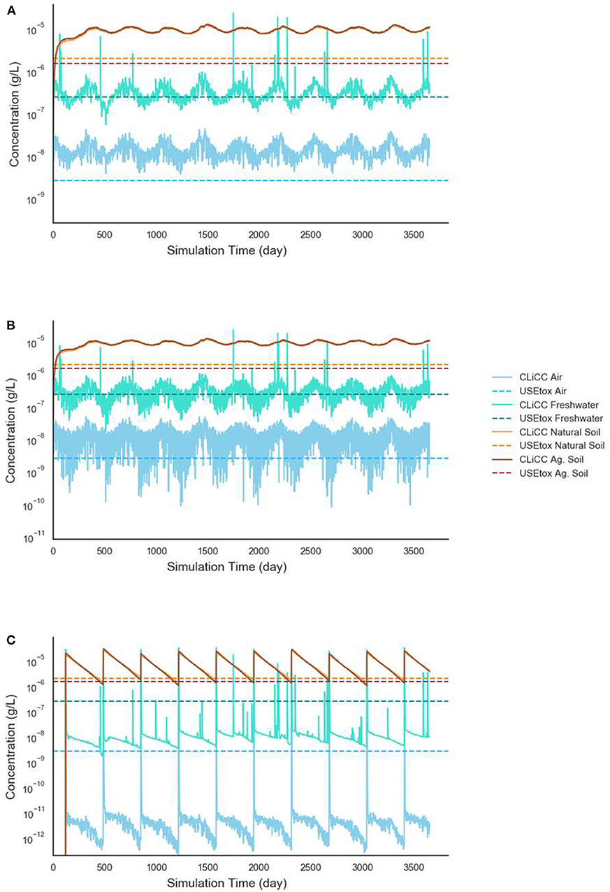
Figure 1. Environmental concentration estimates from CLiCC suite and USEtox 2.1 for 1,2,4,5-tetrachlorobenzene at 100 kt per year emission. (A) Constant emission; (B) workday emission; (C) pulse emission.

Emission profiles

We constructed three emission profiles, each over a 10-year period with emissions entering the air compartment of the environmental system: (1) constant emission, (2) workday emission, and (3) pulse emission. Within each emission profile, three emission magnitudes were used: 10 t/yr, 1, and 100 kt/yr (t stands for metric ton and kt stands for a kilo metric ton). For context, in 2015, the United States production volumes for phthalic anhydride, ethylbenzene, and propargyl alcohol are estimated to be 280, 6,800, and 2.5 kt, respectively (U.S. EPA, 2019a). Before it was banned, there was about 3.2 kt of Aroclor 1254 produced in the United States in 1974 (Agency for Toxic Substances & Disease Registry, 2000). For the constant emission profile, the total emission was evenly spread across each of the days in a year; for workday emission, the total emission was spread over 5 workdays with the 2 weekend days having no emission each week; for pulse emission, the emission was assumed to be released only on May 1st each year, with each pulse being one tenth of the total emission.

Comparison of the outputs

Under the CLiCC suite, daily concentrations of chemicals in various environmental compartments were calculated by ChemFate. Exposure factors through ingestion of the chemicals from all environmental compartments were extracted from those in USEtox 2.1 to keep the comparison as consistent as possible. The reference doses from the IRIS database were used as the threshold exposure level for ingestion. Inhalation exposure was not considered in the case study because the threshold levels for inhalation (reference concentrations) are not readily available for all chemicals in the case study. Values of ED₅₀ for non-cancer effect via ingestion from USEtox 2.1 were used to calculate both the default effect factors in USEtox and the dynamic effect factors described in Equation (4). These intermediate outputs were then applied to the calculation steps described before (Equations 1–5) to arrive at the total impacts due to the emission profiles in this case study. Alternatively, we also used the default effect factors from USEtox to calculate the total impact I_T (cases) for chemical i but with consideration of the threshold levels to examine the deviation from the original outputs from USEtox. This was done as follows:

\begin{array}{l} I_{T, i} = \sum_{t = 0}^{T} X_{E, t, i} \times B W \times E F_{U S E t o x, i} & (6) \end{array}

where BW is the human body weight with a default value of 70 kg and EF_USEtox,i is the default effect factor for non-cancer effect via ingestion [cases/kg_intake] from USEtox.

USEtox 2.1 was modified based on the aforementioned environmental parameters in the Visalia region for the continental scale. Details can be found in Supplementary Material Part 3. USEtox cannot accommodate non-constant emission profiles, hence, only the constant three emission magnitudes were simulated in the modified USEtox model in the case study for environmental concentrations, population exposures, and impact results for this case study. While environmental concentrations and impact results are direct outputs from USEtox, the daily exposure dose for chemical i, X_USEtox,i [mg_chemical/kg_bodyweight-day], is not directly generated from the USEtox model, but can be calculated as follows:

\begin{array}{l} X_{U S E t o x, i} = \frac{i F_{i} \times E M_{i}}{B W \times N_{p o p}} & (7) \end{array}

where iF_i is the intake fraction [kg_intake/kg_emitted] and EM_i is the emission rate [kg_emitted/day] for chemical i. Since intake fraction in USEtox accounts for the population intake from all three scales (urban, continental, and global), we manually set the population of urban scale and global scale to 0 for consistent comparison with our proposed framework, which has one defined scale.

Results

Environmental Concentrations

Table 1 shows the comparison of the outputs from USEtox and CLiCC suite for the constant emission profile with annual emission of 100 kt of chemicals, with the value for CLiCC suite being the average across the 10-year period. Overall, the outputs from the two models are shown to move in the same directions under the constant emission profiles, while the estimates from CLiCC suite are often higher than those from USEtox. The differences across all environmental compartments and chemicals are mostly within a factor of three, with a few larger differences up to around a factor of six. In both models the environmental concentrations scale with the emission magnitude linearly (see Supplementary Material Part 2, Supplementary Table 2.2).

TABLE 1

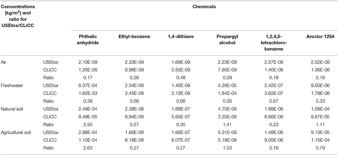
Table 1. Chemical environmental concentration estimates from USEtox and CLiCC suite for the constant emission profile with annual emission of 100 kt.

Figure 1 shows the comparison between environmental concentration estimates from CLiCC suite and USEtox for 1,2,4,5-tetrachlorobenzene in all three emission profiles at 100 kt annual emission. Estimates from USEtox are the same for all emission profiles due to its incapability of accommodating non-constant emissions. For both constant and workday emission profiles, estimates from CLiCC suite reach a semi-steady state rapidly and fluctuate around the average within each year of estimate, reflecting the temporal variations in the environment. For the pulse emission profile, estimates from CLiCC suite show large spikes immediately after the emission events and then steady declines. This also makes estimated concentrations in days when no pulse emission happens substantially lower compared to other emission profiles. Interestingly, estimates of concentrations in the freshwater compartment from CLiCC suite spike irregularly throughout the 10-year period for all emission profiles. This is due to sporadic events of large precipitation occurred in the simulated time period causing a greater than usual transfer of chemicals from the air to the freshwater by an increased rate of deposition. Supplementary Figures 2.1–5 in Supplementary Material Part 2 show the estimated concentrations for all other chemicals with all emission profiles at an annual emission of 100 kt (other emission magnitudes are not shown for brevity, as their shapes are the same since estimates scale with the magnitude of emission linearly).

Daily Exposure Doses

Figure 2 shows the comparison between estimated exposure via ingestion from CLiCC suite and USEtox for 1,2,4,5-tetrachlorobenzene in all three emission profiles at 100 kt annual emission. There are no variations among different emission profiles for estimates from USEtox due to its inherent model structure. For estimates from CLiCC suite, the dynamic of the daily exposure closely resembles the estimated environmental concentration in air. This is because above-the-ground produce is the largest contributor to the total exposure via ingestion and mainly determined by the deposited chemicals from air. The average estimated daily exposure from CLiCC suite is about 4.5 times that of USEtox for both constant and workday emission scenarios but about 3.6 times that of USEtox for pulse emission scenario. Again, the main driver of this difference is the difference in air concentration estimates from the two models as shown in Table 1. For other chemicals, the average daily exposure dose estimates from CLiCC suite are generally higher than that from USEtox by 4–349%. More details can be found in Supplementary Table 2.3 and Supplementary Figures 2.6–10 in Supplementary Material Part 2.

FIGURE 2

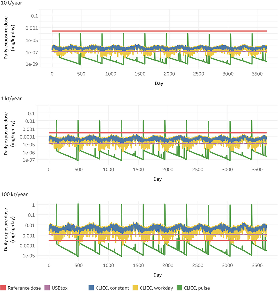
Figure 2. Daily exposure estimates from CLiCC suite and USEtox 2.1 for 1,2,4,5-tetrachlorobenzene.

Effect Factors

Supplementary Figures 2.11–16 in the Supplementary Material Part 2 show the exposure-response curves of all chemicals in the case study, based on Equation (4) and the ED₅₀provided by USEtox for each chemical. They represent cumulative logistic normal probability distributions of the response in the population depending on the exposure that can then be translated into the effect factor after accounting for the population size. The marginal increases in responses for exposure in all curves are small at low concentration levels, sharply accelerating in the middle of the curve, and then reaching plateau when the response is close to 100%. Analytically, the maximum marginal increase in response occurs at an exposure dose of:

\begin{array}{l} X_{E} = e^{log {E D}_{50} - ln 10 \times {σ_{log, e}}^{2}} & (8) \end{array}

which numerically is about 70% of the ED₅₀. This indicates that by using a linearly extrapolated effect factor from 50% response rate would greatly overestimate the human health impact when the population are exposed to low doses of chemicals, which may be the most relevant exposure levels in reality.

Total Human Health Impact

Figure 3 shows the comparison of human health impact estimates between CLiCC suite and original USEtox not considering the threshold assumption. USEtox results are used as reference and CLiCC suite results are shown as a percentage of the reference. The complete results of the human health impact estimates from USEtox and CLiCC with linear and non-linear effect assumptions for all emission profiles and magnitudes along with an interpretation can be found in Supplementary Table 2.4 in the Supplementary Material Part 2.

FIGURE 3

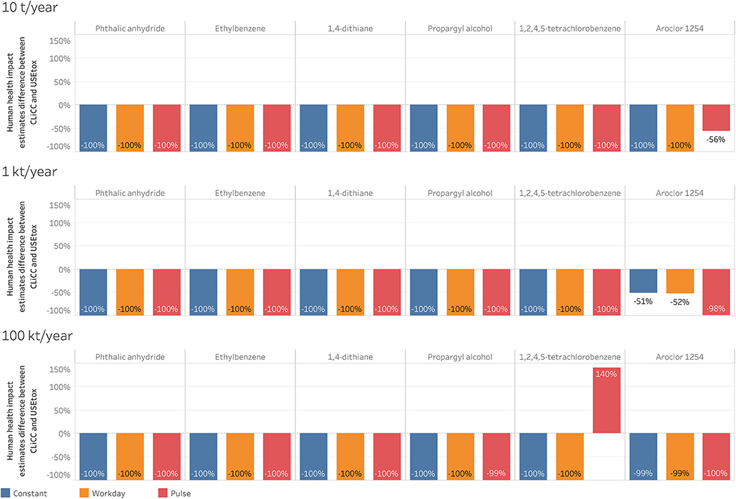
Figure 3. Comparison of human health impact estimates from CLiCC suite to USEtox 2.1 with differences from CLiCC to USEtox shown in percentages as (CLiCC - USEtox)/USEtox × 100%. Toxicity of chemical increases from left to right.

Compared to USEtox, human health impact estimates from CLiCC suite for chemicals with lower toxicity are effectively zero because exposures rarely exceed the reference doses if ever under the simulation conditions in this case study (see Supplementary Figures 2.6–9 in the Supplementary Material Part 2). For the most toxic chemical in the case study, Aroclor 1254, under 10 t/year emission magnitude, both constant and workday emissions result in exposure higher than the reference dose. However, this exposure is not substantial enough to register meaningful impact with the dynamic effect factor: the exposure doses are still on the very left end of the exposure-response curve where marginal increase in response is minimal. Meanwhile, spikes of exposure for the pulse emission result in meaningful impact. With an annual emission of 1 kt, exposures exceed the reference doses substantially for all three emission profiles. However, due to a lower exposure overtime for the pulse emission, its impact is estimated to be much smaller than constant and workday emissions, which are both about half of the estimates from USEtox. With an annual emission magnitude of 100 kt, results of Aroclor 1254 from CLiCC suite for all emission profiles are <1% of the results from USEtox. This is not because the impact estimates from CLiCC suite are low but because with a linear effect factor, the number of cases of disease estimated by USEtox is 28 times higher than the total population in the region, which is unrealistically high (see more in Supplementary Figure 2.10 and Supplementary Table 2.4 in Supplementary Material Part 2). While USEtox impact results are almost always higher than CLiCC suite results despite the exposure estimates are lower than CLiCC suite, there is an exception with 1,2,4,5- tetrachlorobenzene for pulse emission at an annual emission of 100 kt. This is because under this emission profile the exposure exceeds the reference dose meaningfully with the dynamic effect factor to exhibit a significant impact. And with the average daily exposure dose almost 3 times higher than USEtox estimate, the estimated impact becomes higher than USEtox estimate.

Discussion

To our knowledge, this work is the first attempt that compares the results from (1) steady-state and (2) non-linear, dynamic modeling approaches to human health characterization in LCA. Under the constant emission scenario, the results are more comparable between the two approaches. However, when the emission rates fluctuate over time, the results from the two approaches deviate dramatically.

On the one hand, compared with the steady-state model, the dynamic model generally exhibits much lower human health impacts for the constant and workday emission profiles. We believe that the absence of effect thresholds and the current practice of using a fixed slope factor for the exposure-response curve in conventional characterization models run the risk of overestimating the human health impacts from constant ambient emissions below thresholds. This could also lead to unrealistically high results as shown in the results for Aroclor 1254 with an annual emission of 100 kt.

On the other hand, the dynamic approach could lead to higher characterized results as compared to the steady-state counterpart, when it comes to pulse emissions. This is because the peaks in exposure due to pulse emissions may exceed threshold levels, while constant and workday emissions may not, even when their total sums of exposure over time are higher than that of pulse emissions. Our results suggest that conventional characterization practices that average emission rates over time may underestimate the impact from pulse emissions.

The characterization factors derived from non-linear characterization models of CLiCC suite dynamically change in response to the magnitude of emissions, in contrast to their conventional counterparts that are fixed. Despite the difference, the non-linear characterization approach from CLiCC evaluated in this study, in our opinion, conform with the ISO 14044 standard (ISO, 2006), which states that the characterization factors are “derived from a characterization model” and “applied to convert an assigned life cycle inventory analysis result to the common unit of the category indicator.” The ISO 14040 series, to our knowledge, do not require characterization factors to be constant or derived from a linearized model. In some cases, non-linear characterization models and the characterization factors derived from such models may provide a better ground for justification as required by the clause 4.4.2.2.1 of the ISO 14044 standard.

Our study highlights several areas of future research. Along with constant emissions, characterization modeling in LCA often assumes an infinite time horizon. The use of infinite time horizon in characterization without the consideration of no-effect thresholds, however, poses the risk of overestimating the human health impacts of persistent chemicals, as the impact of such chemicals would accrue for decades after the emissions, even if their concentrations in the environment diminish below no-effect thresholds. This problem should be further explored considering both the persistence and toxicity of the chemicals.

When adopting a no-effect threshold for non-cancer effects, however, it is important to consider the level of background exposure, which is usually unspecified, as it could determine whether the marginal increase of emission would push exposure above threshold and reach categorically different conclusions.

In addition, the LCI is generally presented per functional unit without the information on the absolute amount of aggregated emissions to a region. As a result, emissions are usually assumed to be dispersed homogenously across a large region, while in reality, they may be concentrated in a much smaller space. This could underestimate exposures, especially those that are beneath the no-effect threshold when calculated under the assumption of homogenous dispersion, and therefore materially distort the characterization results. Our case study and the models presented along with it offer a starting point to address these challenges in LCIA modeling. In addition, enabling fully dynamic modeling for characterization would require dynamic emission profiles, which are not available in current LCI databases.

Finally, we employed hypothetical values in our case study to evaluate the conditions under which the differences in linear and non-linear models are highlighted. More realistic parameters for e.g., emission rates and background exposure levels will be needed to evaluate the magnitude of the differences between the two modeling approaches under typical conditions. Second, the ability to model non-homogeneous dispersion of emissions across multiple regions and to incorporate inhalation as an exposure route would take the non-steady state fate and transport model employed in our study into the next level.

Data Availability Statement

All datasets generated for this study are included in the article/Supplementary Material.

Author Contributions

DL and MT performed the model calculation. JV reviewed relevant literature. DL, MT, and SS analyzed the results. DL and SS wrote the manuscript. All authors reviewed the manuscript. All authors contributed to the article and approved the submitted version.

Funding

This work was supported by the U.S. Environmental Protection Agency (US EPA) through Science to Achieve Results (STAR) Program Grant No. 83557907. Any opinions, findings, and conclusions or recommendations expressed in this material are those of the authors and do not necessarily reflect the views of US EPA. This work has not been subjected to US EPA review, and no official endorsement should be inferred.

Conflict of Interest

MT is currently employed by the company Amazon.com, Inc., however, the work was done prior to joining Amazon.

The remaining authors declare that the research was conducted in the absence of any commercial or financial relationships that could be construed as a potential conflict of interest.

Supplementary Material

The Supplementary Material for this article can be found online at: https://www.frontiersin.org/articles/10.3389/frsus.2020.569385/full#supplementary-material

References

Agency for Toxic Substances & Disease Registry (editor) (2000). “Production, import, use, and disposal,” in Toxicological Profile for Polychlorinated Biphenyls (PCBs) (Atlanta, GA: U.S. Department of Health and Human Services, Public Health Service), 467–475. Avaialble online at: https://www.atsdr.cdc.gov/toxprofiles/tp.asp?id=142&tid=26

Google Scholar

Boulay, A.-M., Bulle, C., Bayart, J.-B., Deschênes, L., and Margni, M. (2011). Regional characterization of freshwater use in lca: modeling direct impacts on human health. Environ. Sci. Technol. 45, 8948–8957. doi: 10.1021/es1030883

PubMed Abstract | CrossRef Full Text | Google Scholar

Chaudhary, A., Verones, F., de Baan, L., and Hellweg, S. (2015). Quantifying land use impacts on biodiversity: combining species–area models and vulnerability indicators. Environ. Sci. Technol. 49, 9987–9995. doi: 10.1021/acs.est.5b02507

PubMed Abstract | CrossRef Full Text | Google Scholar

Djomo, S. N., Knudsen, M. T., Andersen, M. S., and Hermansen, J. E. (2017). Methods for regionalization of impacts of non-toxic air pollutants in life-cycle assessments often tell a consistent story. Atmospheric Environ. 169, 218–228. doi: 10.1016/j.atmosenv.2017.09.018

CrossRef Full Text | Google Scholar

Dong, Y., Rosenbaum, R. K., and Hauschild, M. Z. (2016). Assessment of metal toxicity in marine ecosystems: comparative toxicity potentials for nine cationic metals in coastal seawater. Environ. Sci. Technol. 50, 269–278. doi: 10.1021/acs.est.5b01625

PubMed Abstract | CrossRef Full Text | Google Scholar

Fantke, P., Bijster, M., Guignard, C., Hauschild, M., Huijbregts, M., Jolliet, O., et al. (2017a). USEtox^® 2.0 Documentation (Version 1). Available online at: http://usetox.org

Google Scholar

Fantke, P., Jolliet, O., Apte, J. S., Hodas, N., Evans, J., Weschler, C. J., et al. (2017b). Characterizing aggregated exposure to primary particulate matter: recommended intake fractions for indoor and outdoor sources. Environ. Sci. Technol. 51, 9089–9100. doi: 10.1021/acs.est.7b02589

PubMed Abstract | CrossRef Full Text | Google Scholar

Fantke, P., McKone, T. E., Tainio, M., Jolliet, O., Apte, J. S., Stylianou, K. S., et al. (2019). Global effect factors for exposure to fine particulate matter. Environ. Sci. Technol. 53, 6855–6868. doi: 10.1021/acs.est.9b01800

CrossRef Full Text | Google Scholar

Huijbregts, M. A. J., Rombouts, L. J. A., Ragas, A. M. J., and van de Meent, D. (2005). Human-toxicological effect and damage factors of carcinogenic and noncarcinogenic chemicals for life cycle impact assessment. Integr. Environ.Assess. Manag. 1, 181–244. doi: 10.1897/2004-007R.1

PubMed Abstract | CrossRef Full Text | Google Scholar

ISO (2006). Environmental management—Life cycle Assessment—Requirements and Guidelines. ISO 14044: 2006. Geneva: ISO.

Google Scholar

Levasseur, A., Lesage, P., Margni, M., Deschênes, L., and Samson, R. (2010). Considering Time in LCA: dynamic LCA and its application to global warming impact assessments. Environ. Sci. Technol. 44, 3169–3174. doi: 10.1021/es9030003

PubMed Abstract | CrossRef Full Text | Google Scholar

Levasseur, A., Lesage, P., Margni, M., and Samson, R. (2013). Biogenic carbon and temporary storage addressed with dynamic life cycle assessment. J. Indus. Ecol. 17, 117–128. doi: 10.1111/j.1530-9290.2012.00503.x

CrossRef Full Text | Google Scholar

Motoshita, M., Itsubo, N., and Inaba, A. (2011). Development of impact factors on damage to health by infectious diseases caused by domestic water scarcity. Int. J. Life Cycle Assess. 16, 65–73. doi: 10.1007/s11367-010-0236-8

CrossRef Full Text | Google Scholar

Roy, P.-O., Azevedo, L. B., Margni, M., van Zelm, R., Deschênes, L., and Huijbregts, M. A. J. (2014). Characterization factors for terrestrial acidification at the global scale: a systematic analysis of spatial variability and uncertainty. Sci. Total Environ. 500–501, 270–276. doi: 10.1016/j.scitotenv.2014.08.099

PubMed Abstract | CrossRef Full Text | Google Scholar

Seppäl,ä, J., Posch, M., Johansson, M., and Hettelingh, J.-P. (2006). Country-dependent characterisation factors for acidification and terrestrial eutrophication based on accumulated exceedance as an impact category indicator. Int. J. Life. Cycle Assess. 11, 403–416. doi: 10.1065/lca2005.06.215

CrossRef Full Text | Google Scholar

Shah, V. P., and Ries, R. J. (2009). A characterization model with spatial and temporal resolution for life cycle impact assessment of photochemical precursors in the United States. Int. J. Life Cycle Assess. 14, 313–327. doi: 10.1007/s11367-009-0084-6

CrossRef Full Text | Google Scholar

Slob, W., and Pieters, M. N. (1998). A probabilistic approach for deriving acceptable human intake limits and human health risks from toxicological studies: general framework. Risk Anal. 18, 787–798. doi: 10.1111/j.1539-6924.1998.tb01121.x

PubMed Abstract | CrossRef Full Text | Google Scholar

Struijs, J., van Dijk, A., Slaper, H., van Wijnen, H. J., Velders, G. J. M., Chaplin, G., et al. (2010). Spatial- and time-explicit human damage modeling of ozone depleting substances in life cycle impact assessment. Environ. Sci. Technol. 44, 204–209. doi: 10.1021/es9017865

PubMed Abstract | CrossRef Full Text | Google Scholar

Tao, M., and Keller, A. A. (2020). ChemFate: a fate and transport modeling framework for evaluating radically different chemicals under comparable conditions. Chemosphere 255:126897. doi: 10.1016/j.chemosphere.2020.126897

PubMed Abstract | CrossRef Full Text | Google Scholar

U.S. EPA (2019a). 2016 Chemical Data Reporting Results. US EPA. Available online at: https://www.epa.gov/chemical-data-reporting/2016-chemical-data-reporting-results (accessed November 6, 2019).

Google Scholar

U.S. EPA (2019b). Integrated Risk Information System. Available online at: https://www.epa.gov/iris (accessed September 26, 2019).

Google Scholar

van Zelm, R., Huijbregts, M. A. J., van Jaarsveld, H. A., Reinds, G. J., de Zwart, D., Struijs, J., et al. (2007). Time horizon dependent characterization factors for acidification in life-cycle assessment based on forest plant species occurrence in europe. Environ. Sci. Technol. 41, 922–927. doi: 10.1021/es061433q

PubMed Abstract | CrossRef Full Text | Google Scholar

Verones, F., Saner, D., Pfister, S., Baisero, D., Rondinini, C., and Hellweg, S. (2013). Effects of consumptive water use on biodiversity in wetlands of international importance. Environ. Sci. Technol. 47, 12248–12257. doi: 10.1021/es403635j

PubMed Abstract | CrossRef Full Text | Google Scholar

Keywords: non-linearity, human health, characterization, life cycle impact assessment, chemicals

Citation: Li D, Tao M, Vieira J and Suh S (2020) The Effects of Incorporating Non-linearity in LCA: Characterizing the Impact on Human Health. Front. Sustain. 1:569385. doi: 10.3389/frsus.2020.569385

Received: 03 June 2020; Accepted: 03 September 2020;
Published: 07 October 2020.

Edited by:

Reinout Heijungs, Vrije Universiteit Amsterdam, Netherlands

Reviewed by:

Lei Huang, University of Michigan, United States
Giovanni Mondello, University of Messina, Italy

Copyright © 2020 Li, Tao, Vieira and Suh. This is an open-access article distributed under the terms of the Creative Commons Attribution License (CC BY). The use, distribution or reproduction in other forums is permitted, provided the original author(s) and the copyright owner(s) are credited and that the original publication in this journal is cited, in accordance with accepted academic practice. No use, distribution or reproduction is permitted which does not comply with these terms.

*Correspondence: Sangwon Suh, suh@bren.ucsb.edu

^†Present address: Mengya Tao, Amazon.com, Inc., Seattle, WA, United States Jessica Vieira, Apeel Sciences, Goleta, CA, United States

ORIGINAL RESEARCH article

The Effects of Incorporating Non-linearity in LCA: Characterizing the Impact on Human Health

Introduction

Materials and Methods

The CLiCC Suite

Overview

Dynamic Fate and Transport Model

Characterization Factor Calculation

Case Study

Case Study Setup

Chemicals

Landscape environmental and climate data

Emission profiles

Comparison of the outputs

Results

Environmental Concentrations

Daily Exposure Doses

Effect Factors

Total Human Health Impact

Discussion

Data Availability Statement

Author Contributions

Funding

Conflict of Interest

Supplementary Material

References

This article is part of the Research Topic

People also looked at