A River of Bones: Wildebeest Skeletons Leave a Legacy of Mass Mortality in the Mara River, Kenya

Introduction

Animals can have myriad effects on biogeochemistry, nutrient cycling, and ecosystem function through both direct and indirect effects on trophic processes and through transport processes (Bauer and Hoye, 2014; Schmitz et al., 2018). Animals tend to aggregate in time and space, which can lead to biogeochemical hot spots and hot moments (McClain et al., 2003), and animals can move across ecosystem boundaries, which can transport resource-rich subsidies against natural gradients or at an elevated rate along natural gradients (Subalusky and Post, 2018). Live animals can play important roles in driving these dynamics through nutrient assimilation and excretion, during which animals can serve as sinks for some elements by assimilating them in their body tissue (Kitchell et al., 1979; Atkinson et al., 2016; Nobre et al., 2019). After death, animal carcasses may play an important role as a nutrient source by liberating limiting nutrients (Bump et al., 2009; Beasley et al., 2012; Keenan et al., 2018).

Animal carcasses provide a complex and heterogeneous resource for an array of consumers. Animal carcasses can result from annual or seasonal mortality associated with normal life history, selective drivers of mortality (e.g., disease, predation, hunting), or mass mortality events (Wilmers et al., 2003; Ameca y Juárez et al., 2012; Fey et al., 2015; Wenger et al., 2019). The resulting differences in the abundance, location, and timing of carcass deposition, as well as in animal characteristics including body size and stoichiometry, can have pronounced effects on decomposition and utilization of carcass components (Tomberlin and Adler, 1998; Beasley et al., 2012; Subalusky and Post, 2018). Carcass decomposition is a multi-stage process: an early stage of decomposition characterized by high rates of elemental leaching, an active stage characterized by microbial and insect colonization, and an advanced stage characterized by physical/mechanical breakdown and chemical dissolution of bones (Parmenter and Lamarra, 1991; Keenan et al., 2018). The earlier stages can be relatively rapid, occurring over days to months, as compared to the latter stage, as bones can persist for decades to millennia (Vereshchagin, 1974; Smith and Baco, 2003; Miller, 2011; Miller et al., 2013).

Much research has focused on the influence of soft tissues, which provide the majority of carcass resources for invertebrates and small-bodied vertebrates. Soft tissues are high in nitrogen (N) and phosphorus (P), which are often limiting nutrients in ecosystems. The stoichiometric ratio of N to P in soft tissues ranges from 10 to 100:1 (Elser et al., 1996). Soft tissues decompose over days to weeks, but they can have pronounced and rapid ecological effects that can persist for long periods of time (Parmenter and Lamarra, 1991; Chaloner et al., 2002; Regester and Whiles, 2006; Bump et al., 2009; Parmenter and MacMahon, 2009; Pray et al., 2009).

Much less research has focused on the decomposition and utilization of bones from animal carcasses (Wambuguh, 2008; Wenger et al., 2019). Bone is a composite material consisting of a mineral phase, an organic phase, and water (Currey, 2002). The mineral phase is comprised of calcium phosphate primarily in the form of hydroxylapatite. The organic phase is comprised of collagen, non-collagenous proteins, and lipids. As a result of this structure, bones have a much higher proportion of P than soft tissues, with N:P ratios of < 1:1 (Elser et al., 1996; Subalusky et al., 2017), and bones can persist in ecosystems for decadal time scales (Smith and Baco, 2003; Wenger et al., 2019). Because the scaling of bone and body size in terrestrial vertebrates is non-linear, larger-bodied vertebrates have a much larger proportion of their total body mass comprised of bone than small-bodied animals (Prange et al., 1979; Elser et al., 1996). Altogether, these studies suggest bones may provide a long-term, P-rich resource, particularly when bones result from carcasses of large vertebrates, raising questions about the role they may play in nutrient cycling and consumer dynamics.

The fate of bones in an ecosystem is largely influenced by environmental context. Bones in terrestrial ecosystems are subject to decomposition via exposure to sun and rain, fungus, and foraging by animals that can consume bones, including rodents and larger animals such as hyenas. Bone persistence in tropical, terrestrial ecosystems is on the scale of several decades (Behrensmeyer, 1978; Trueman et al., 2004; Western and Behrensmeyer, 2009; Ross and Cunningham, 2011). Bone decomposition in temperate and arctic latitudes, which are cooler and drier, can extend over millennial time scales (Vereshchagin, 1974; Andrews, 1995; Wambuguh, 2008; Miller, 2011; Michelutti et al., 2013). In marine ecosystems, the limited role of bacteria and the temporal stability of environmental conditions can result in slow decomposition rates that foster the development of specialist assemblages on carcasses (Baco and Smith, 2003; Smith and Baco, 2003; Beasley et al., 2012). Bone decomposition in aquatic ecosystems may be slowed by occasional burial in benthic sediments (Johnston et al., 2004). Studies suggest only 10–15% of fish bone may be lost due to permanent burial (Vallentyne, 1960; Schenau and De Lange, 2000; Vanni et al., 2013), although this rate likely varies widely depending on characteristics of the aquatic ecosystem and has not been well-studied. Despite these burial rates, accumulation of detritus from fish bones in marine benthic sediments can comprise a significant portion of sediment P and lead to high rates of phosphate fluxes under certain conditions (Schenau and De Lange, 2001).

Aquatic ecosystems likely have higher densities of bones than terrestrial ecosystems because, in addition to mortality of aquatic vertebrates, they may also be a source of mortality for terrestrial animals as well as aggregate slowly-decomposing bones from the terrestrial landscape (Behrensmeyer, 1982; Wenger et al., 2019). There is a long history of studying the origin and persistence of bonebeds and fluvial transport of bones in paleoecology (Behrensmeyer, 1988, 2007). However, little work has focused on the potential ecological effects of bones in aquatic ecosystems. The disparity in the amount of ecological research on carcasses versus that on bones is illustrated in a Web of Science search conducted on 14 March 2019 for literature on the topic. Studies on carcass decomposition in aquatic ecosystems [(carcass OR body) AND (decomposition OR decay) AND aquatic] since 1990 yielded 218 studies, as compared to a search for studies on bone decomposition [(bone OR skeleton) AND (decomposition OR decay) AND aquatic] that yielded only 25 studies (Figure 1).

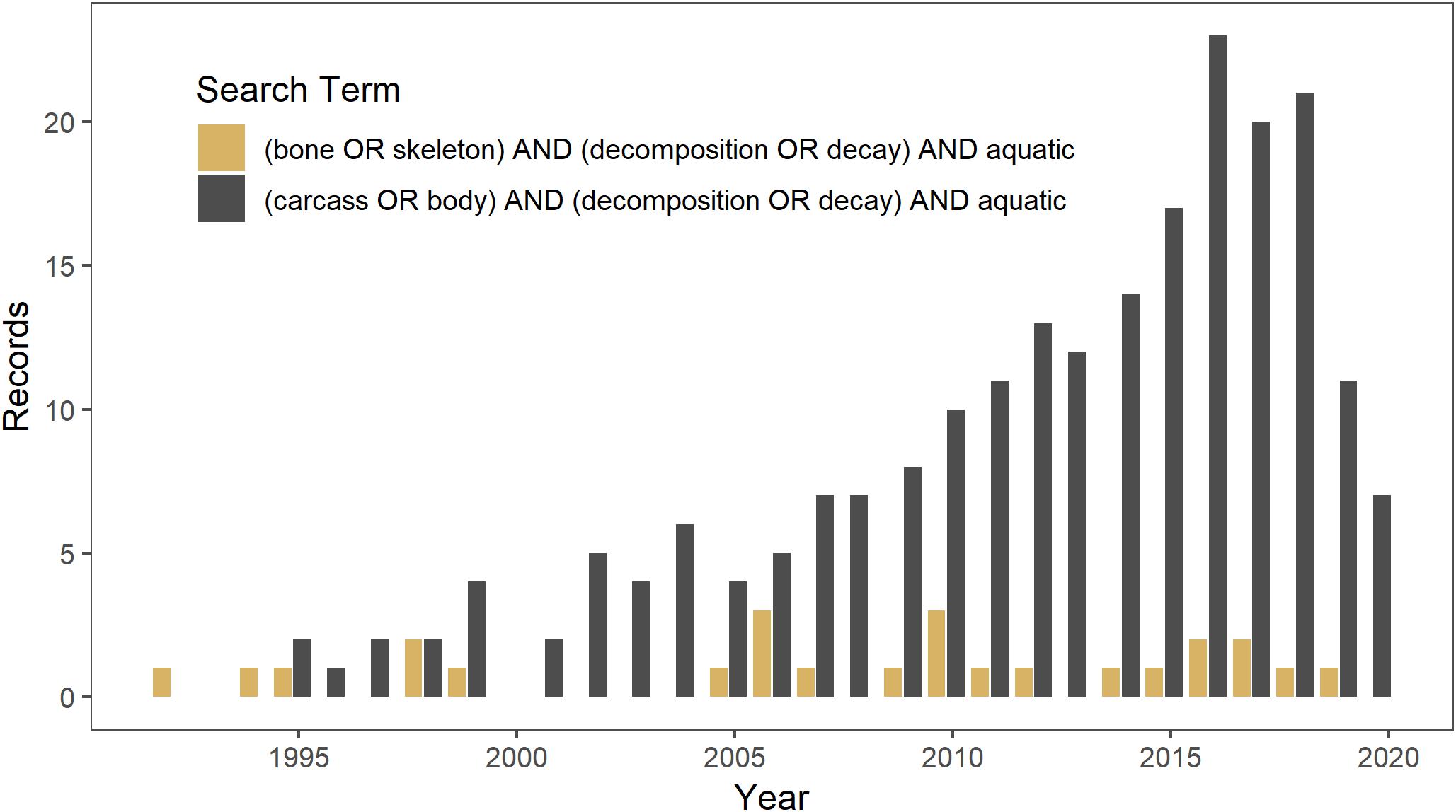
Figure 1. Web of Science search conducted on 14 March 2019 for literature since 1990 on decomposition in aquatic ecosystems of carcasses (in gray) versus bones (in brown).

The Serengeti wildebeest (Connochaetes taurinus) migration provides an opportunity to examine the influence of large inputs of bones from large mammals on river ecosystem function, and raises interesting questions about the ontogeny and effects of animal bones in aquatic ecosystems (Figure 2). Annual mass drownings in the Mara River result in the input of an average of 6,250 carcasses into the river every year (Subalusky et al., 2017). Approximately half of a wildebeest carcass is soft tissue, which decomposes over weeks to months, but the other half is bone, which comprises 95% of the phosphorus (P) in a carcass and decomposes over years (Subalusky et al., 2017). The pulsed input of these carcasses influences nutrient cycling in the river on annual time scales (Subalusky et al., 2017, 2018), but there may also be long-term effects on nutrient cycling and river food web dynamics through the persistence of bones.

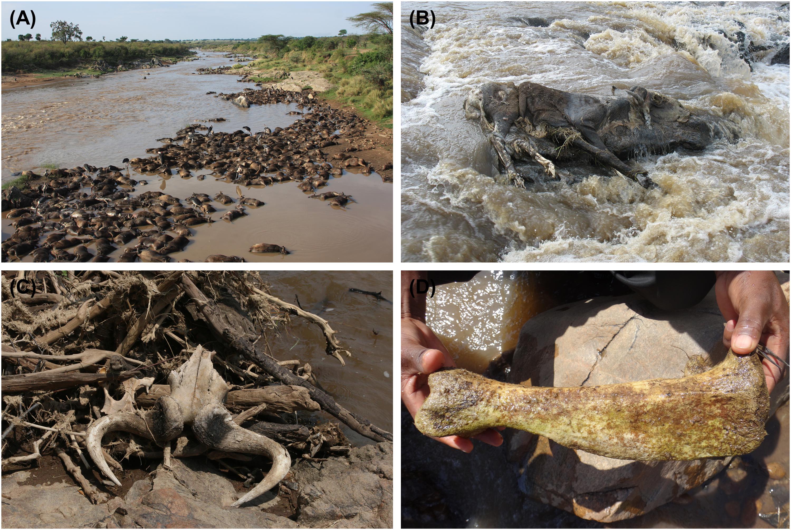
Figure 2. The ontogeny of wildebeest bones in the Mara River, Kenya. (A) Annual mass drownings result in the input of a mean of 6,250 carcasses per year. (B) Carcass soft tissue decomposes over weeks to months, but bone persists in the river for decades. (C) Bones can continue to leach out phosphorus even after a prolonged period in the river. (D) Biofilms that grow on bones are higher in chl a and organic matter (OM) than biofilms on rocks, and they provide an important food source for macroinvertebrates and fishes.

Here we synthesize several datasets from our research in the Mara River to examine the ecological effects that bone could have on nutrient cycling, ecosystem function, and food web structure in the river. We use these data and our preliminary understanding of the role of bones in this ecosystem to propose several research questions to improve our broader understanding of the role of mammal bones in aquatic ecosystems. We also suggest this may be an overlooked phenomenon in other rivers and may have been particularly important in the past when robust populations of large mammals were more common.

Materials and Methods

Study Site

This research took place in the Mara River, which runs through the Maasai Mara National Reserve in Kenya and the Serengeti National Park in Tanzania. The river hosts a population of > 4,000 hippopotamus (Hippopotamus amphibius) and the annual migration of 1.3 million wildebeest, which both provide important resource subsidies to the river (Subalusky et al., 2015, 2017). The Serengeti wildebeest migration is in the Kenyan portion of the Mara River basin from July to November, and the animals cross the Mara River multiple times during this period as they move between dry season feeding grounds. We have documented nearly annual mass drownings of wildebeest during river crossings upstream of the New Mara Bridge near the border between Kenya and Tanzania (Subalusky et al., 2017).

From 2011 to 2015, we estimated a mean of 6,250 wildebeest drowned in the river each year, which contributed approximately 219,200 kg of bones (wet weight) per year to the river (Subalusky et al., 2017). All but one of these drownings occurred within a 5 km reach of river, and carcasses tend to accumulate on river bends and rock outcroppings within a 5 km reach downstream of the drowning location. Thus, if we assume these bones are distributed along a 10 km reach, and the average river width is 40 m, these annual inputs would yield an areal density of 0.55 kg bone/m². This estimate does not account for the continual accrual of bones that occurs due to their slow decomposition, and it does not account for the transport of bones farther downstream that likely occurs over time.

All data presented in this paper were from samples collected just upstream of the New Mara Bridge, which is ∼200 m upstream of the Tanzanian border, or from an artificial stream experiment that was conducted inside the Maasai Mara National Reserve. All wildebeest bones were collected from the carcasses of animals that drowned naturally in the river. Fishes were sampled using standard field methods. This study was carried out in accordance with the Yale University Institutional Animal Care and Use Committee Animal Use Protocol #2012-10734.

Bone Decomposition

We measured bone decomposition using three different approaches: (1) measuring in situ mass loss of bones in litterbags in the river, (2) measuring changes in the elemental composition of bones after an extended time in the river, and (3) measuring nutrient leaching rates from bones in microcosms.

First, we placed samples of four different types of fresh bone (triplicate samples of leg, rib, scapula, vertebrae; n = 12) inside fine mesh (<500 μm) litterbags that were secured inside a metal cage in the river. We measured wet mass at five time intervals (between days 0 and 216), and we replaced the same bone samples in the bags after weighing. We did not destructively sample bone for dry mass because of considerable heterogeneity both within and across bone types and difficulty in obtaining a homogenous sample. We calculated decay rate in the R package litterfitter (Cornwell and Weedon, 2014; Cornwell et al., 2014), which allowed us to use AIC model selection to compare a single-pool exponential decay model (Eq. 1), which assumes a homogenous sample with a single decay rate, with a two-pool exponential decay model (Eq. 2), which fits initial mass distributions and parallel decay rates for a sample composed of two different components (e.g., labile and recalcitrant) (Manzoni et al., 2012; Cornwell and Weedon, 2014).

In both equations, M₀ is the mass remaining at time 0, M_t is the mass remaining at time t, and t is time to decomposition in days. In Eq. 1, k is the constant decomposition rate of the material. In Eq. 2, ∝ is the proportion of labile material, k₁ is the decomposition rate of labile material, and k₂ is the decomposition rate of recalcitrant material. All models were run for 500 iterations. We used the resulting parameter values for the selected model to estimate time to 95% mass loss as ln(0.05)/k for the labile and recalcitrant components.

We also used these parameter values to calculate the steady-state standing stock of bones in the Mara River, according to the following equation:

In this equation, I is the annual input of bones scaled to a daily rate (600.5 kg wet mass day⁻¹), and ∝, k₁, and k₂ are from Eq. 2 (Cornwell and Weedon, 2014).

Second, we compared the carbon (C), nitrogen (N), and phosphorus (P) composition of bone samples that were collected fresh (triplicate samples of rib, vertebrae, and joint bones; n = 9) with those collected after 216 days of litterbag deployment in the river (triplicate samples of leg, rib, scapula, vertebrae; n = 12). Bone samples were dried at 72°C (to meet USDA permit import regulations), lightly sanded to remove any connective tissue from the surface, and finely ground using a cryogenic ball mill. C and N composition were measured using a Costech Elemental Analyzer (Costech Analytical Technologies, Inc., Valencia, CA, United States). P composition was measured by digesting pre-weighed, combusted material using 1M HCl at 80°C for 2 h, treating with an ammonium molybdate color reagent, and analyzing on a flow analyzer (Astoria-Pacific, Clackamas, OR, United States). The percent organic matter (OM) was measured by weighing samples before and after combustion. We used t-tests to compare the % OM, % C, % N, and % P in fresh bones versus aged bones of different types (R Core Team, 2018). We compared fresh rib, vertebrae, and joint bones to aged rib, vertebrae, and leg bones, respectively.

Third, we measured initial leaching rates of bone by placing sub-samples of fresh bone (66–98 g, mean = 80 g) in chambers (n = 3) that were filled with 4 L of unfiltered river water and open to the environment. We collected 50 mL water samples for analysis of inorganic nutrients every ∼6 days for 31 days. Water samples were collected using a syringe and filtered through a 0.2 μm Supor polysulfone filter (Pall Corporation, Port Washington, NY, United States) into a sample bottle and frozen until analysis. Samples were analyzed on a portable flow injection analyzer in the field. Ammonium was analyzed using the gas exchange method (APHA, 2006). Nitrate was analyzed using zinc reduction (Ellis et al., 2011). Soluble reactive phosphate (SRP) was analyzed using the molybdate blue method (APHA, 2006). Nutrient concentrations were multiplied by the volume of water in the chamber at each sampling time point to obtain total mass of nutrients leached. We did not correct for background nutrient concentrations in the water we used to fill the chambers, as we did not maintain control chambers over time, but concentrations were very low compared to leaching rates of ammonium and SRP. The mass of the bone sample was multiplied by the % N and % P measured for fresh joint bones, and the ammonium and SRP that leached out over 31 days was measured as a proportion of the total N and P in the bone sample.

Effects of Bones on Ecosystem Function in Experimental Streams

As part of a larger mesocosm experiment examining the influence of wildlife subsidies on ecosystem function, we used recirculating experimental streams to compare the influence of bone versus rock substrates on water column nutrient concentrations, and water column and benthic production. Details of the experimental stream array are in Subalusky et al. (2018). In this experiment, we had 18 individual streams (three blocks of six streams each), and treatments were randomly assigned among each block. The full experiment included controls (n = 4), and four different treatments (n = 2–4). We only present here data from the control streams (n = 4) and the bone treatment streams (n = 2).

One 5-L bucket of washed gravel was placed along the bottom of each stream channel as substrate, and five ceramic tiles were placed in the channel bed for sampling. Streams were filled with 60 L water from Emarti Bridge, which is on the Mara River upstream of the influence of large wildlife, and inoculated with periphyton scrubbed from rocks from New Mara Bridge, within the range of wildlife. Streams were allowed to equilibrate for 1 week, after which treatments were applied, and the experiment was run for two additional weeks. In the bone treatment streams, half of the volume of gravel was replaced with wildebeest bones of unknown age that had been removed from the river. This treatment had approximately 0.7 kg bones m^–2, which is comparable to our estimates of areal density of bones in the Mara River.

We used a Manta2 sonde (Eureka Environmental, Austin, TX, United States) containing a Cyclops-7F submersible fluorometer (Turner Designs, San Jose, CA, United States) to measure water column chlorophyll a (chl a) weekly. We collected water samples weekly to analyze inorganic nutrients, as described above. We also destructively sampled one ceramic tile each week to measure OM of the biofilm as ash free dry mass (AFDM). We filtered a known volume of sample through a pre-weighed, pre-combusted Whatman GF/F filter (GE Healthcare Bio-Sciences, Pittsburgh, PA, United States), and measured AFDM by drying the filter at 60°C, re-weighing it, combusting it for 4 h at 450°C and then re-weighing it to determine mass loss upon combustion. In the final week of the experiment, we scrubbed the biofilm off one ceramic tile from each stream and measured the concentration of chl a in a known volume of water using the Manta2 sonde, which we then converted to chl a per unit area of tile. In situ chl a fluorescence can be used as a proxy for chl a concentration, although it may provide an overestimate, and direct comparison with chl a concentrations requires calibration (Holm-Hansen et al., 2000; Roesler et al., 2017). However, in this analysis, we only compared in situ fluorescence values across treatments.

Data were analyzed for normality using a Shapiro–Wilk’s normality test in R Core Team (2018), and water column nutrients, water column chl a, and benthic AFDM were log-transformed to meet statistical assumptions. We examined differences in water column nutrients, water column chl a, and benthic AFDM throughout the duration of the experiment using a linear mixed-effect model run with the lme function in the nlme package in Pinheiro et al. (2016) and R Core Team (2018). We fitted lme models with the restricted maximum likelihood method and a continuous autoregressive temporal correlation structure with week as the repeated factor. Treatment (control, bone) and time (each of 3 weeks of measurement) were treated as fixed effects, and individual streams were treated as random effects. We then used the lsmeans package to perform a Tukey pairwise comparison test between treatments for parameters over the duration of the experiment (Lenth, 2016; R Core Team, 2018). We also analyzed the effect of treatment on biofilm chl a at the end of the experiment with a one-way ANOVA using the aov function in R Core Team (2018).

Bone Biofilm

We analyzed chl a and OM (measured as AFDM) of biofilms collected from both wildebeest bones and rocks in the Mara River in November 2013 (during the wet season) and February 2014 (during the dry season). At both sampling times, we selected three rocks and three bones from the same reach of river, scrubbed the entire upper surface of the substrate clean using a toothbrush, and analyzed photos of the substrates using ImageJ software to measure the surface area (Schneider et al., 2012). We filtered a known volume of sample through a pre-weighed, pre-combusted Whatman GF/F filter, and measured AFDM as described above. We filtered a known volume of sample through a second Whatman GF/F filter for analysis of chl a. We froze the filter paper for > 24 h, extracted the chl a using methanol with a basic pH (Holm-Hansen, 1978), and analyzed the samples on a Turner Aquafluor handheld fluorometer (Turner Designs, San Jose, CA, United States). We calculated both chl a and AFDM per unit surface area of the substrate. Data were tested for normality using a Shapiro–Wilk’s normality test in R, and we analyzed the effect of substrate and season on both parameters using a two-way ANOVA with the aov function followed by a Tukey HSD test in R Core Team (2018).

We analyzed community composition of biofilms from both wildebeest bones and rocks collected from the Mara River in October 2017 and November 2018. In 2017, we scrubbed biofilms from the surfaces of three bones and three rocks randomly selected from the same reach of river, although sampling was not done quantitatively. Samples were preserved with Lugol’s solution and counted in the lab at 400x on a Leica DM LS2 compound microscope until 100 algal cells had been reached, and abundance of each taxa was given as a proportion of the total. In 2018, we collected three bones and three rocks from the same reach of river, making sure to collect paired samples from similar depths, and scrubbed 16 cm² of surface area. Samples were again preserved with Lugol’s solution and counted in the lab. We counted 10 microscope fields for each sample, and we calculated the total abundance of each taxa. We identified both bone and rock periphyton to phylum (Chlorophyta, Chrysophyta, Cyanobacteria, Euglenozoa) (Prescott, 1978), and we parsed Chlorophyta into three functional groups based on growth form (unicellular, colonial, and filamentous). We conducted an analysis of similarity on the community data separately for each year using the anosim function in the vegan package in R Core Team (2018) and Oksanen et al. (2019). The function vegdist is used to create a Bray dissimilarity matrix, and anosim uses the rank order of dissimilarity values to test for statistically significant differences between communities.

Stable Isotopes

We used C and N stable isotopes to examine isotopic differences between biofilms on rocks and biofilms on bones over three different seasons. We collected biofilms from rocks and bones in November 2013 (wet season), February 2014 (dry season), and July 2016 (wet season) (n = 3 of each type in each season). We also analyzed the stable isotope signature of fresh wildebeest bones (n = 8) collected in 2012–2013 to help interpret differences in biofilm signature between bones and rocks. We then used C and N stable isotopes to partition the contribution of various basal food web resources to the tissue assimilation of aquatic macroinvertebrates and fishes. We used sample data from February 2014, as this was 4 months after any fresh wildebeest carcasses were in the river. This time period should exceed the typical isotope turnover rate for consumer muscle tissue (Vander Zanden et al., 2015) and thus minimize the signal of wildebeest carcass soft tissue in the consumers. We used biofilms growing on rocks and on bones to characterize autochthonous basal food web resources, and we collected samples of hippo feces (n = 9), which is the primary source of allochthonous food web resources in this region of the river (Masese et al., 2015; Subalusky et al., 2015, 2018).

We collected 16–30 individuals from each of four families of aquatic macroinvertebrates, including Baetidae, Hydropsychidae, Caenidae, and Simulidae, and we combined individuals into a single bulk sample per family. For Baetidae and Simulidae, we had sufficient individuals to run two replicate samples of 30 individuals each, and we used the mean of those replicates for the stable isotope signatures of those taxa. We also collected tissue samples from the lateral muscle of three species of fishes, including Labeo victorianus (n = 8), Labeobarbus altianalis (n = 5), and Bagrus docmac (n = 3). All samples were collected from near the New Mara Bridge. All samples were dried, ground into a fine powder, and analyzed for δ¹³C and δ¹⁵N on a ThermoFinnigan Delta Plus Advantage stable-isotope mass spectrometer (Thermo Scientific, Boca Raton, FL, United States) coupled to a Costech ECS 4010 Elemental Analyzer (Costech Analytical Technologies, Inc., Valencia, CA, United States).

We used Bayesian mixing models in MixSIAR to estimate the proportion of each basal resource assimilated in macroinvertebrate and fish tissue (Moore and Semmens, 2008; Stock and Semmens, 2013). The results of fish assimilation were analyzed and presented by species in Subalusky et al. (2017); here, we analyzed assimilation across aquatic macroinvertebrates and fishes as composite consumer groups. All fish species were omnivorous, so we used 0.4 ± 1.3 for δ¹³C (Post, 2002) and 4.3 ± 1.5 for δ¹⁵N (Bunn et al., 2013) for fish trophic enrichment factors, which incorporates variability in trophic structure. We used 0.4 ± 1.3 for δ¹³C (Post, 2002) and 1.4 ± 1.4 for δ¹⁵N (Bunn et al., 2013) for macroinvertebrate trophic enrichment factors. We ran models with the normal MCMC parameters (100,000 chain length, 50,000 burn-in). Visual analysis of isospace plots confirmed that consumer data were within the minimum convex polygon of source data, suggesting we were not missing any major diet sources (Phillips et al., 2014).

Results

Bone Decomposition

The in situ decomposition of bone in the Mara River was much better described by the two-pool model of decomposition than by the single-pool model for all four bone types (Table 1). Results from this model suggest different bone types vary in their decomposition rate. Bones are comprised of 7–27% labile material that decomposes over 78–119 days, and 73–93% refractory material that decomposes over > 80 years (Table 1). The k value for the refractory material in all bone types reached the minimum bounds in this analysis package (0.0001), providing a minimum estimate for the time to 95% loss; however, extrapolation beyond this time point is well outside the bounds of what we can infer with the relatively limited duration of our field data (216 days). Scapula and leg bones had the lowest proportion of labile material and as a result decomposed the most slowly (Figure 3). Vertebrae bones had the highest proportion of labile material and decomposed more quickly than the other bone types. It is unlikely that bone mass loss during this experiment was due to downstream transport of particulate material, due to the fine mesh size of the litterbags used. Based on an annual input of 219,200 kg (wet mass), we estimate the steady-state standing stock of bones in the Mara River is 4.4 × 10⁶ to 5.6 × 10⁶ kg. This estimate is likely high, as it assumes the system is in equilibrium, and it is based on a conservative decay rate due to microbial decomposition that does not account for loss from animal consumption or mechanical breakdown.

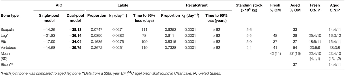
Table 1. Comparison of single- and dual-pool negative exponential models of decomposition for four different wildebeest bone types, parameter values for the best fit model (AIC values in bold; the dual-pool model was the best fit for all bone types), estimates of time to 95% loss for labile and recalcitrant material, and overall% organic matter (OM) and C:N:P stoichiometry by percent mass for wildebeest bones after 216 days in the river and a bison skull after 1000s of years underwater.

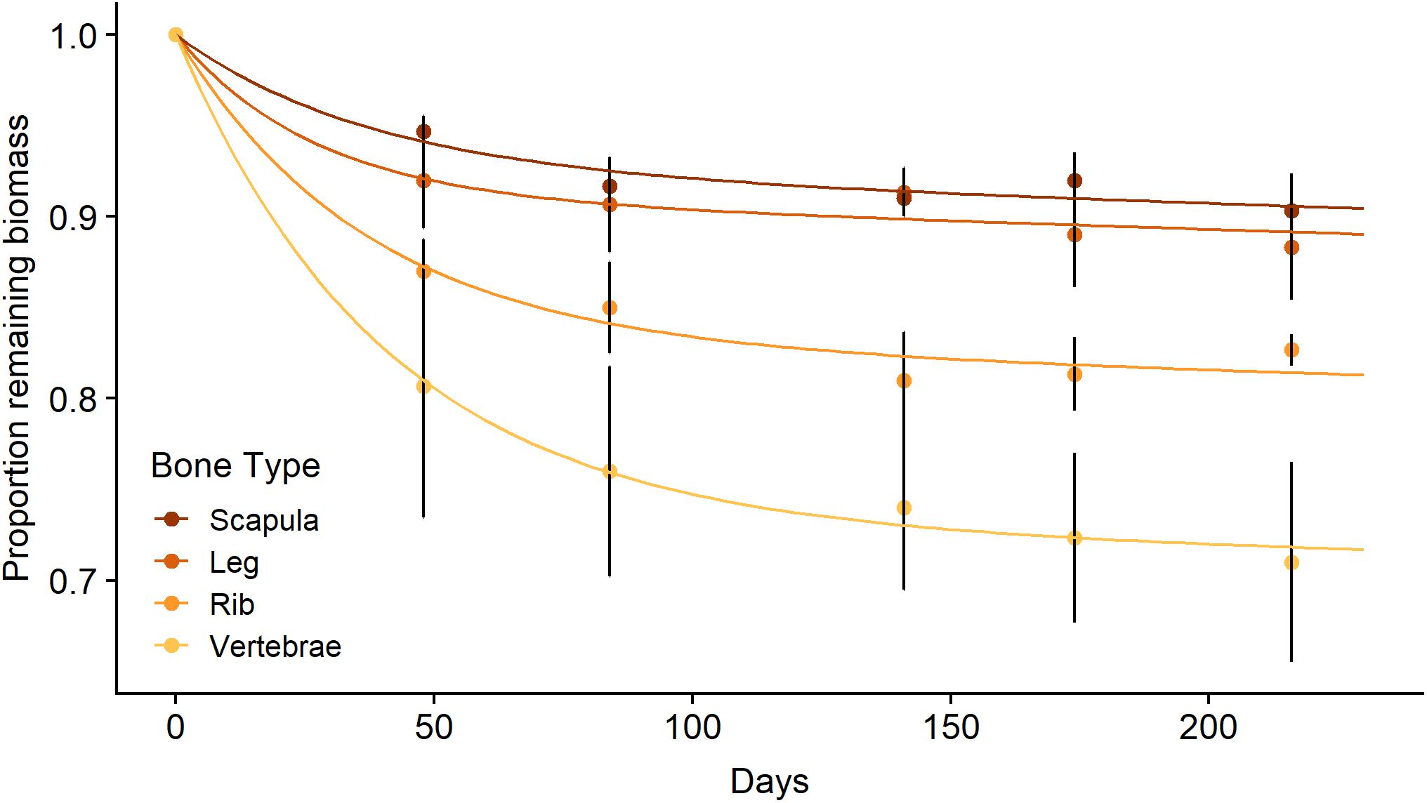
Figure 3. Mean (± SE) proportion of biomass remaining for scapula, leg, rib, and vertebrae bones (n = 3 per bone type) from a wildebeest carcass during litterbag deployment in the Mara River with best fit models following a parallel discrete model of decomposition.

There were relatively small differences in the stoichiometry of fresh versus aged bones (those that had been in the river for 216 days) (Figure 4 and Table 1). The mean % OM decreased on average from 42 ± 11% in fresh bones to 37 ± 16% in aged bones. The average stoichiometry of fresh bones (joint, rib, and vertebrae) was 22.1 C: 4.5 N: 9.9 P by % mass compared to 23.1 C: 3.5 N: 10.2 P for aged bones. In leg and rib bones, the % C and % N declined, while the % P increased, likely due to the relatively higher % C and N of labile material in bone (e.g., lipids) and the higher % P of refractory material (e.g., apatite). However, in vertebrae, % C increased as % N and % P decreased over time, which may reflect a greater degree of vascularization and greater initial proportion of labile N and P in this bone type. The only significant changes were the decrease in % N in rib bones (t-test, t = −6.5₃.₂, p = 0.006) and the increase in % P in leg bones (t = −4.25₃.₉, p = 0.014) (Figure 4).

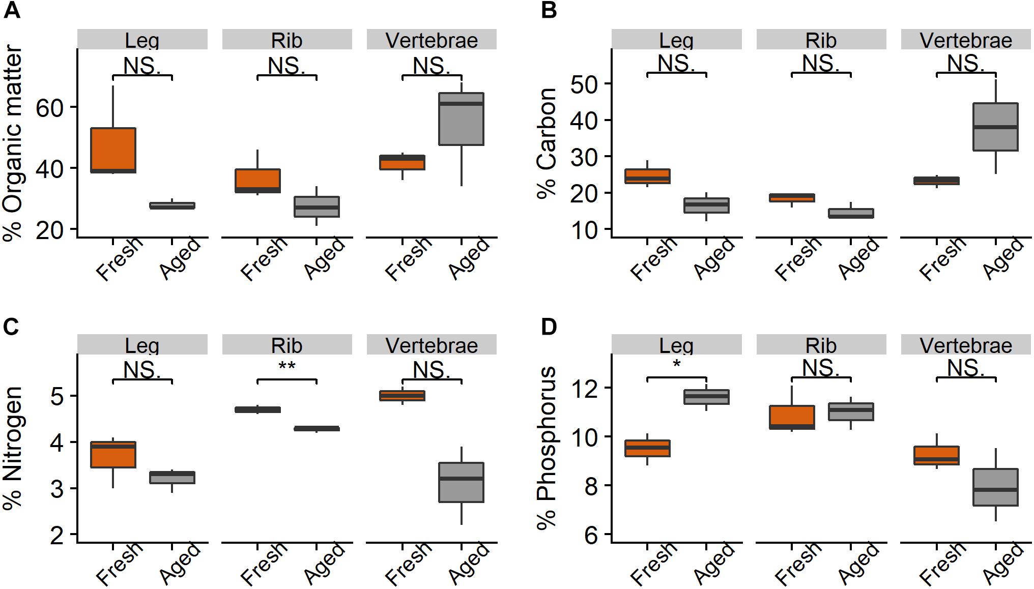
Figure 4. Percent (A) organic matter, (B) carbon, (C) nitrogen, and (D) phosphorus in leg, rib, and vertebrae bones (n = 3 per bone type) from wildebeest when fresh and after 216 days in the Mara River. Fresh joint bone was compared to aged leg bone. Asterisks indicate significant difference, where *p < 0.05 and **p < 0.01.

In the chamber experiment, approximately 50% of the mass of SRP and ammonium that leached out of the bones over a month was available after only 3 days (Figure 5). The mass of ammonium that leached out after 1 month (96.8 ± 35.7 mg, mean ± SD) was almost an order of magnitude larger than that of SRP (12.7 ± 2.9 mg). Background values from the water used in the chambers (SRP = 0.16 mg, NH₄ = 0.50 mg) were ∼1% of the final values. Ammonium appeared to stabilize during the latter half of the month, which may have been due to equilibration with the atmosphere, while SRP continued to increase. A large amount of nitrate available on day 1 (5.0 ± 0.3 mg) was due to the water used in the chamber, which had a background nitrate value of 4.8 mg, but nitrate levels fell to nearly zero by day 3 and stayed there for the duration of the study. This decline was likely due to loss through denitrification due to anoxic conditions in the mesocosms, which we did not measure. We also did not measure other forms of nutrient uptake that may have occurred in these chambers; thus, our estimates of leaching rates are likely conservative. After 31 days, we estimate the bone samples leached out 3.2 ± 0.7% (mean ± SD) of the initial N as ammonium and 0.2 ± 0.0% of the initial P as SRP.

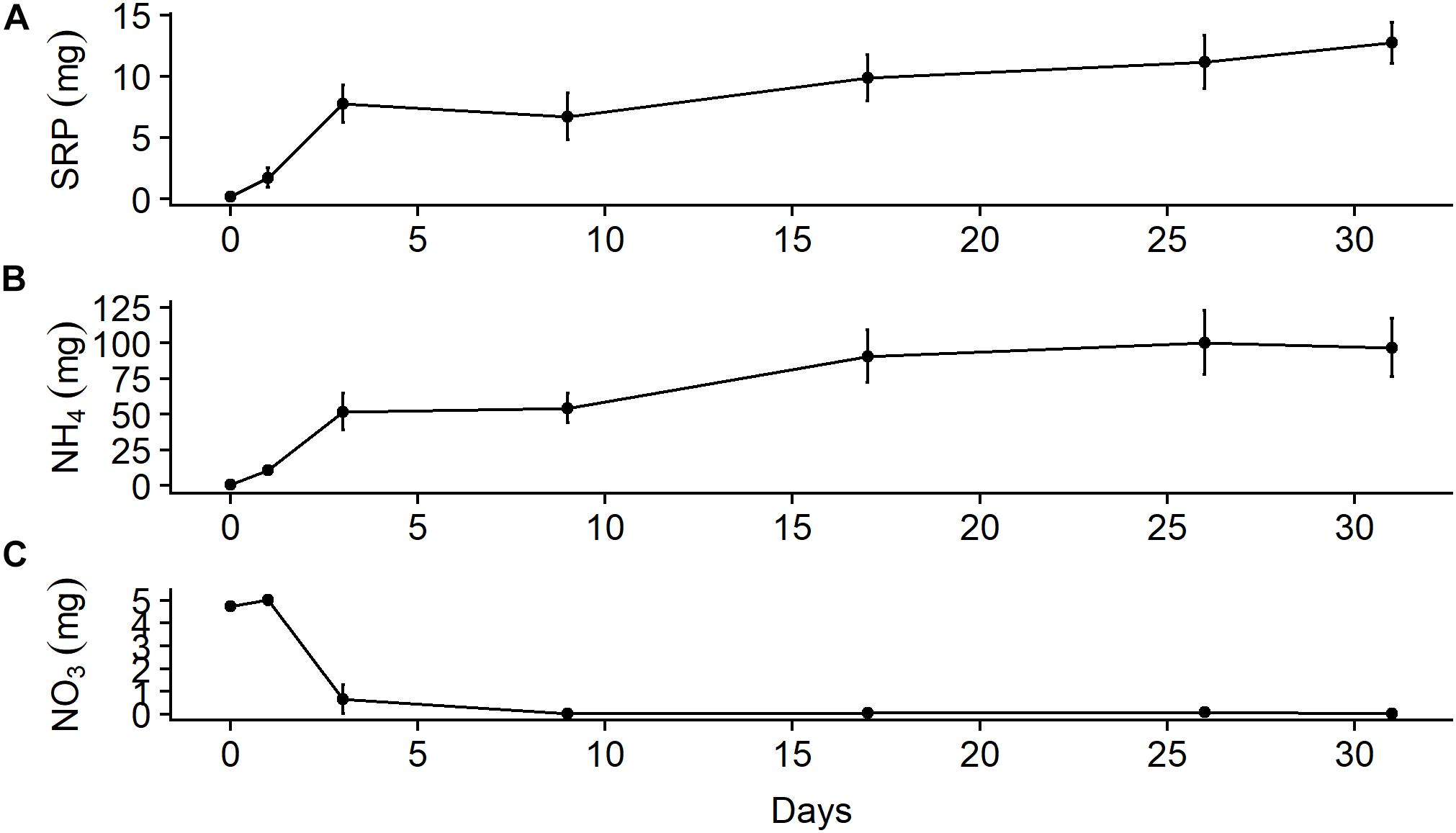
Figure 5. Mean (± SE) total mass in 5-L microcosms (n = 3) filled with river water of (A) soluble reactive phosphorus, (B) ammonium, and (C) nitrate leached out of wildebeest leg bone.

Effects of Bones on Ecosystem Function in Experimental Streams

There was a significant effect of both treatment (LME ANOVA: F₅,₁ = 213.621, p < 0.001) and time (F₅,₂ = 22.547, p < 0.001), and a significant interaction between them (F₅,₂ = 81.530, p < 0.001), on water column SRP in the experimental streams (Figure 6A). There was no difference between the bone treatment and the control in week 1, before treatments were applied, indicating similar background conditions. After the treatments were applied, the bone treatment had > 300 times higher SRP than the control treatment in week 2 (p < 0.001) and 150 times higher in week 3 (p = 0.001) of the experiment.

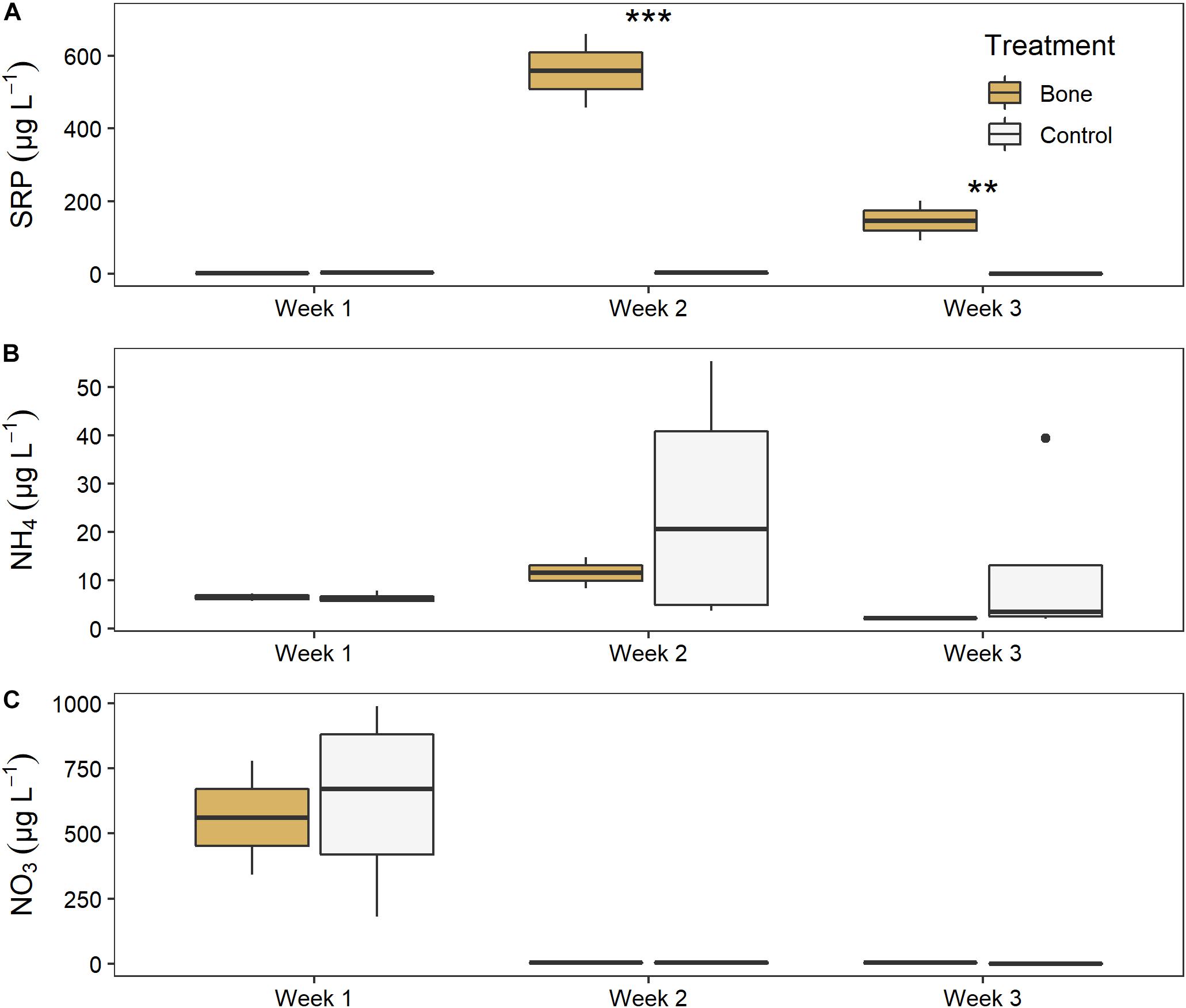
Figure 6. Water column (A) soluble reactive phosphorus, (B) ammonium, and (C) nitrate in experimental streams with all gravel benthos (control treatment; n = 4) or half gravel-half bone benthos (bone treatment; n = 2) in Week 1, after equilibration and just before treatments were applied, and in Weeks 2 and 3 of the experiment. Asterisks indicate significant difference, where **p < 0.01 and ***p < 0.001.

There was no significant effect of treatment or time, or significant interactions between them, for ammonium (Figure 6B). There was a significant effect of time on NO₃ (F₅,₂ = 204.075, p < 0.001) although no treatment effect, as both the bone and control treatment declined from ∼600 μg L^–1 NO₃ to nearly zero between weeks 1 and 2 (Figure 6C).

There was no significant effect of treatment on water column chl a in the experimental streams, but there was a significant effect of time (LME ANOVA: F₅,₂ = 9.972, p = 0.007) and a significant interaction between treatment and time (F₅,₂ = 17.369, p = 0.001). Chl a was 5 times higher in the bone treatment (364 ± 32) than the control treatment 70 ± 17) in week 2, although this was not statistically significant (p = 0.0737), likely due to low replication (Figure 7A). There was no difference between the bone and control treatment in week 1 or week 3.

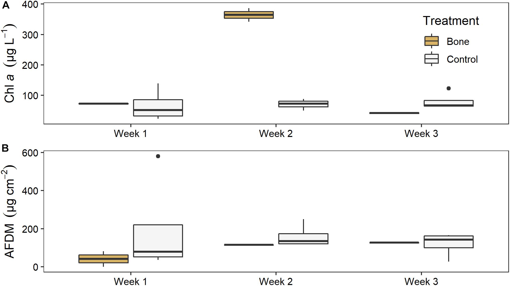
Figure 7. (A) Water column chl a and (B) biofilm ash free dry mass (AFDM) on ceramic tiles in experimental streams with all gravel benthos (control treatment; n = 4) or half gravel-half bone benthos (bone treatment; n = 2) in Week 1, after equilibration and just before treatments were applied, and in Weeks 2 and 3 of the experiment, after treatments were applied.

There was no significant effect of treatment or time, or a significant interaction between them, on tile biofilm AFDM (Figure 7B). There also was no significant effect of treatment on tile biofilm chl a at the end of the artificial stream experiment (ANOVA: F₅,₁ = 0.171, p = 0.7).

Bone Biofilm

Biofilm on bones had significantly higher chl a (two-way ANOVA; F₁,₁₁ = 14.64, p = 0.005) and OM (two-way ANOVA; F₁,₁₁ = 9.13, p = 0.017) than biofilms on rocks (Figure 8). Chl a was 4.6 times higher and AFDM was 2.0 higher on bone biofilm than on rock biofilm. There was no significant effect of season or interaction between season and substrate.

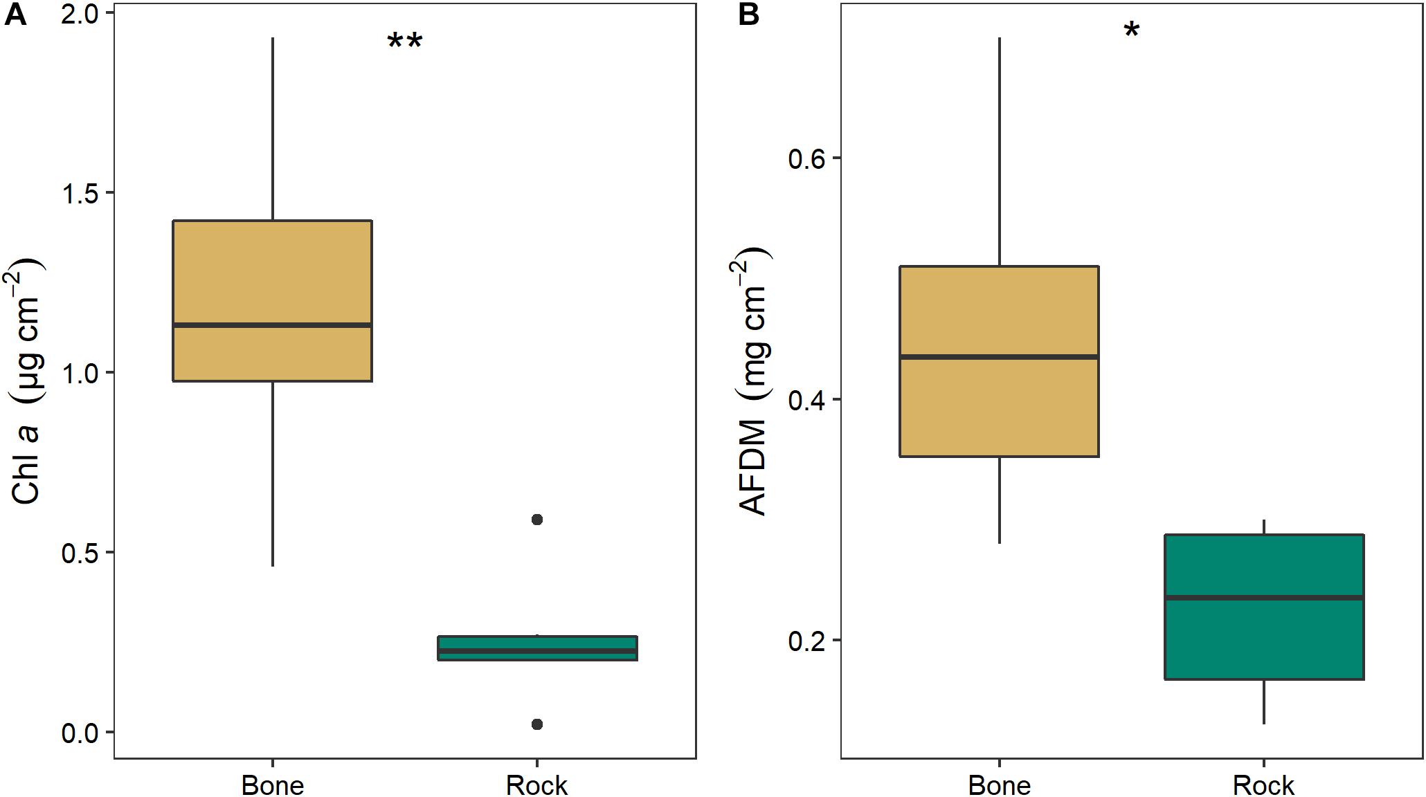
Figure 8. Mean (± SE) values of (A) chlorophyll a and (B) organic matter as ash free dry mass (AFDM) on bone (n = 3) and rock (n = 3) substrates in the Mara River. Asterisks indicate significant difference, where *p < 0.05 and **p < 0.01.

There was no significant difference between the algal communities in biofilms growing on bones and those growing on rocks in either year (2017: ANOSIM R = −0.1481, p = 0.9; 2018: ANOSIM R = −0.1852, p = 0.8). The negative R values indicate greater dissimilarities within groups than between groups (Figure 9). In 2017, unicellular algae were the most common, followed by colonial algae and diatoms. In 2018, diatoms were the most common, followed by filamentous and colonial algae.

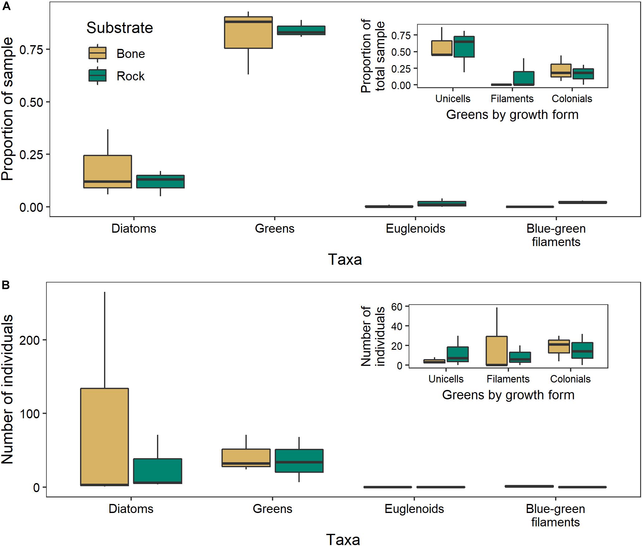
Figure 9. Algal community composition on bone (n = 3) and rock (n = 3) substrates in the Mara River, where individuals are presented as (A) a proportion of 100 individuals counted in 2017, or (B) total number within 10 microscope fields in 2018. Green algae are parsed by growth form in the inset figures.

Stable Isotopes

Biofilm on bones had a δ¹⁵N similar to that of biofilm on rocks (0.4–1.7‰ difference) but a δ¹³C that was much more enriched (4–10‰) (Figure 10). The δ¹³C of biofilm on bones was much closer to the δ¹³C of wildebeest bones themselves (1.6–3.7‰ difference). These data suggest biofilms on both rocks and bones may be obtaining N from the water column, but biofilms on bones may be obtaining some C from the bones themselves.

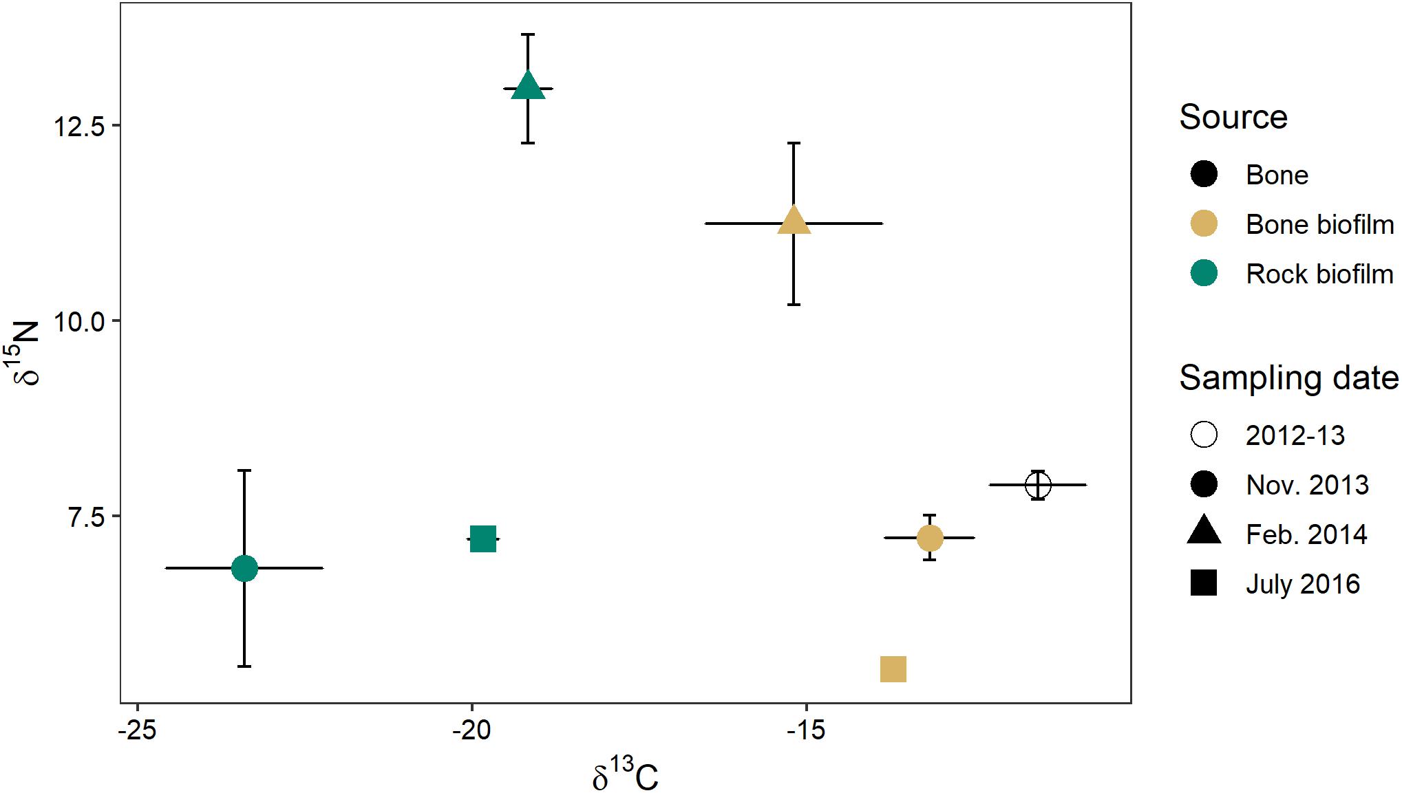
Figure 10. C and N stable isotope signatures of wildebeest bone (n = 8) and biofilm on rock and on bone on three sampling dates (n = 3 of each at each time point) in the Mara River.

Sufficient differences between the three dominant basal resources at NMB in February 2014 (bone biofilm, rock biofilm, and CPOM) enabled us to parse their influence on aquatic consumers (Table 2). Mixing model results showed that bone biofilm accounts for 19 ± 16% (mean ± SD) of assimilated tissue in macroinvertebrates and 24 ± 13% in fishes in the Mara River (Figure 11). These proportions are similar to that of rock biofilm for macroinvertebrates (21 ± 13%), but greater than rock biofilm for fishes (7 ± 6%). The remaining portion of both macroinvertebrate and fish diet is comprised of hippo feces, which accounts for nearly all of the particulate OM at this site. The results support an important contribution of bone; however, we note that the 95% Bayesian credible intervals are quite wide and overlap for most of the resources, indicating a reasonable amount of uncertainty in the contribution.

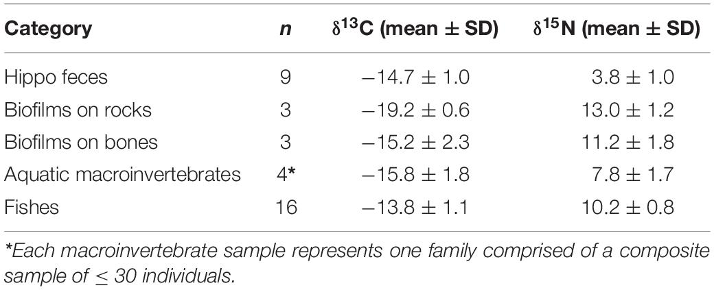
Table 2. Stable isotope signatures of basal food web resources, aquatic macroinvertebrates, and fishes collected in February 2014, at the New Mara Bridge in the Mara River.

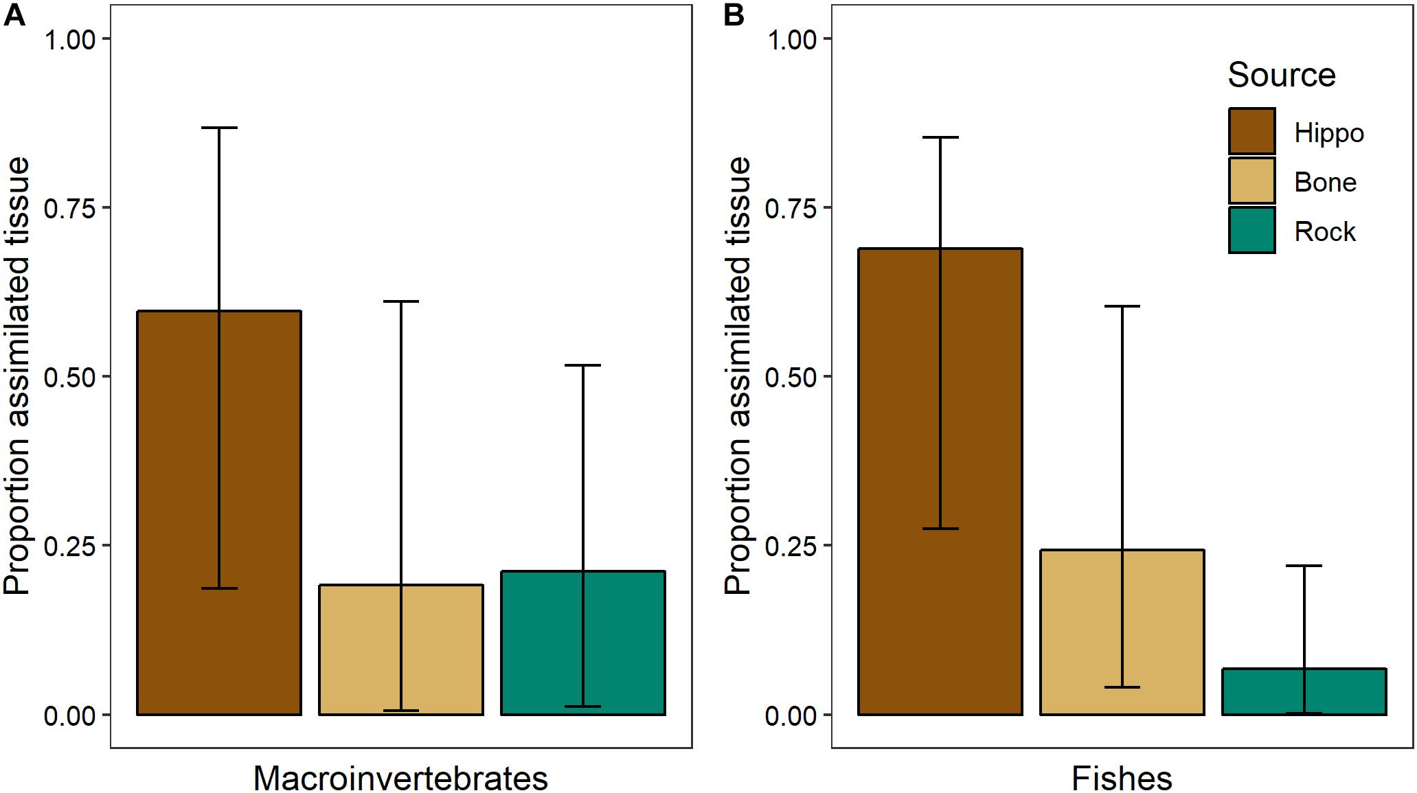
Figure 11. Proportion of basal resources in assimilated tissue (mean and 95% Bayesian credible intervals) of (A) aquatic macroinvertebrates (n = 4 taxa, composite samples of 16–30 individuals/taxa) and (B) fishes (n = 3 taxa, 3–8 individuals/taxa) in February 2014 in the Mara River from hippo feces (n = 9), bone biofilm (n = 3), and rock biofilm (n = 3).

Discussion

Wildebeest bones provide a distinct and complex resource in the Mara River, and given their abundance in this system, they may influence nutrient cycling, ecosystem production, and food web dynamics at the river ecosystem scale. Wildebeest bone is comprised of 22% C, 4% N, and 10% P, although stoichiometry and decomposition rates vary by bone type (Table 1). A mean of 15% of the initial mass of bones is relatively labile and decomposes over 80–120 days (Figure 3). Initial leaching releases a large amount of inorganic N relative to P (Figure 5). After this labile portion is gone, the more refractory material that is rich in P can persist in the system for decades, although mineralization and leaching of P continue to occur. For example, bones that had been submersed in the river for an unknown period of time still released SRP when placed in the experimental stream channels (Figure 6). The increase in SRP during week 2 of the experiment may have reflected either a pulse of SRP release in response to changing environmental conditions between the river and the experimental streams, or a steady release of SRP that declined in week 3 due to uptake. These data suggest that large mammal bones play a unique role as slow-release nutrient subsidies in this system.

Nutrient leaching from bones may stimulate increased production. In the experimental stream channels, the increase in SRP in the bone treatment in week 2 was coincident with five times more water column chl a but no change in tile AFDM (Figure 7), suggesting P from bones stimulated water column primary production. In the river, biofilms growing on bones had five times more chl a and two times more OM than biofilms growing on rocks (Figure 8), suggesting bones may support greater quantity and/or quality of biofilms. Increased biofilm growth on bones could be due to leaching of nutrients from the bones and/or greater surface roughness of bones as compared to rocks, which could provide increased surface area for growth (Bergey and Cooper, 2015). There did not appear to be a difference in algal composition on bones versus rocks (Figure 9).

The isotopic signature varied between biofilms on bones and those on rocks, with the δ¹³C of bone biofilm being closer to that of wildebeest bones themselves (Figure 10). These data suggest some biofilm constituents may be able to utilize elements leaching from the bones, particularly C, which could have implications for bone biofilm quantity and quality. Mixing model analysis suggests aquatic macroinvertebrates and fishes assimilate a similar proportion of bone biofilm, which is equal to or greater than the proportion of rock biofilm assimilated (Figure 11). Given the likely much lower abundance of bones on the river bottom as compared to rocks, these data suggest consumers may be preferentially feeding on biofilms growing on bones. If so, that preference could be driven by higher density or quality of the biofilms growing on bones as compared to those growing on rocks.

Many of these analyses are based on small sample sizes, and we synthesize them here to stimulate areas for future research. Altogether, these data suggest bones may play an important and persistent ecological role in the Mara River, and they raise several over-arching questions about the potential ecological role of bones in aquatic ecosystems in general.

What Is the Magnitude and Frequency of Animal Bone Inputs to Aquatic Ecosystems?

The Mara River receives annual inputs of large mammal bones, and bones persist in this system over long timescales. The large input rate and slow decomposition rate yield a steady-state standing stock estimate of 4.4 × 10⁶ to 5.6 × 10⁶ kg of bones in the river, which is equivalent to the biomass of 49 blue whales. This estimate is likely high, as it assumes that the system is in equilibrium and input rates have been constant over time, and it is based on a conservative decomposition rate that does not account for animal consumption or mechanical breakdown. This estimate also does not reflect the potential distribution of bones downstream through the river system and into the Mara Wetland and Lake Victoria. Nevertheless, it reflects the magnitude of bone that can accrue in a system that receives large inputs of carcasses, particularly of large mammals. How typical is this of other aquatic ecosystems?

Animal bones can enter aquatic ecosystems through various pathways. Wenger et al. (2019) proposed a framework for classifying animal carcass inputs to aquatic ecosystems, in which inputs may be either autochthonous and continuous (e.g., annual mortality from aquatic animals), autochthonous and pulsed (e.g., mass mortality of aquatic animals), allochthonous and continuous (e.g., annual mortality from terrestrial animals that are transported in from the watershed), or allochthonous and pulsed (e.g., seasonal mortality from terrestrial animals that perish in situ). The wildebeest inputs to the Mara River represent an example of allochthonous and pulsed, which has the potential to be one of the largest sources of inputs in certain systems. For example, research building on historical, anecdotal accounts suggests that large-scale inputs of bison bones may have been commonplace in the rivers of the American Great Plains as recently as the late 1700s. A mass drowning of bison in the Assiniboine River could have comprised ∼50% of the annual P load for that river (Saindon, 2003; Wenger et al., 2019). It is unknown how the magnitude of these inputs would compare to those resulting from in situ mortality of aquatic vertebrates, such as fishes. However, allochthonous inputs from terrestrial animals that transport additional resources into the system are likely to have different and perhaps more pronounced ecosystem effects as compared to autochthonous ones (Subalusky and Post, 2018). Furthermore, the size of bones likely influences their stoichiometry and decomposition rate, such that larger bones may be expected to provide the slow release of nutrients we observed with wildebeest bones, whereas smaller bones may decompose more quickly (Nobre et al., 2019). Much work remains to be done to quantify the magnitude of animal carcass inputs from these four categories across ecosystems and over time and space. We expect that rates of allochthonous carcass inputs to aquatic ecosystems would be highest in higher order rivers, which both aggregate more from the watershed and may provide a cause of direct mortality for animals, and in landscapes with abundant populations of large mammals and particularly migratory herds.

How Bioavailable Are the Elements in Bones, and Over What Time Scales Do They Become Available?

Our data suggest most of the labile nutrients leach out of bone within a few months of deposition; however, they also indicate that the recalcitrant nutrients can continue to leach out of bone at longer time scales. Thus, bones have the ability to provide a slow-release nutrient subsidy to aquatic ecosystems, which lengthens the temporal scale at which we normally consider animal influences on nutrient cycling. What are the rates of P mineralization from the recalcitrant portion of bones, and what other elements may be leaching from the bones, such as calcium? How do these mineralization rates change across environmental conditions and over time? And how may the attachment of algae and microbes facilitate the erosion of bones through alteration of the boundary layer pH or scavenging of minerals? Much of the forensic and archeological study of bone decomposition has focused on bones buried in soil, and research suggests increasing soil temperature, moisture content and geochemistry are all important variables in driving microbial decomposition, although a great deal of variability occurs in bones even within the same site (Hedges, 2002; Christensen and Myers, 2011; High et al., 2015). In aquatic ecosystems, where less research has been done on bone decomposition, the decomposition process can be even more variable due to the large number of variables that can influence the process, including temperature, water depth, currents, dissolved oxygen, dissolved OM, substrate type, salinity, acidity, and insect and scavenging activity (Simon et al., 1994; Heaton et al., 2010). In lake and river ecosystems, bone burial in benthic sediments is likely to slow or stop decomposition. Studies of fish bones suggest 10–15% of bones may be permanently buried in lakebed sediments (Vallentyne, 1960; Schenau and De Lange, 2000; Vanni et al., 2013). How do decomposition processes vary across species and ecosystem types, and how bioavailable are elements throughout these processes?

As part of this study, we analyzed the C, N, and P composition of a bison skull that was recently recovered from Clear Lake, IA, United States, in order to understand how extended submersion in an aquatic ecosystem (e.g., over centuries to millennia) could influence bone composition in another species. Modern American bison (Bison bison) have been extirpated from that region for several 100 years; however, preliminary analysis based on the skull’s shape and size suggests this may be a prehistoric specimen (Skinner and Kaisen, 1947). We conducted radiocarbon dating to determine the skull is 3,360 ± 25 years BP (¹⁴C age); thus, this skull could have been in the water for 1000s of years. The bison skull had very similar proportion of OM (37%) and C:N:P stoichiometry (13.7 C: 4.3 N: 10.6 P by % mass) to the fresh rib and aged scapula bones from the wildebeest, suggesting that even bones 100s to 1000s of years old may still retain a fairly large proportion of organic material. In the case of the bison skull, burial in lake sediments in a cold region likely maintained its relatively intact condition.

Are Animal Bones Capable of Influencing Aquatic Ecosystem Function?

Altogether, our data suggest bones may provide important nutrient and microhabitat resources at local scales in this system. However, it is still unclear to what degree these effects scale up to influence the whole river ecosystem. To what degree can long-term mineralization of bone inputs support primary, and ultimately secondary, production in aquatic ecosystems? The answer likely depends upon both the magnitude of the inputs and the environmental context of the aquatic ecosystem (Subalusky and Post, 2018). In the Mara River, wildebeest bones contribute a substantial portion of the annual P flux from upstream (Subalusky et al., 2017). P flux is significantly higher at the site where wildebeest drownings occur, but only when carcasses are present, suggesting long-term leaching of bones does not significantly elevate P flux at the site scale (Subalusky et al., 2018). However, it may be readily assimilated and stimulate primary production, as we observed in the experimental streams. Indeed, water column chl a is higher at the site where drownings occur, although the degree to which that production is due to wildebeest inputs versus other drivers is still unclear (Subalusky et al., 2018). There also may be more localized hotspots of P availability by bone piles that could have ecological consequences. Whole ecosystem effects of wildebeest bones may be muted in the Mara River, where even larger resource subsidies from hippos have pronounced ecosystem effects (Subalusky et al., 2018). However, in systems with substantial inputs of large bones and low background nutrient loading, it is possible that bones could influence ecosystem function over long time scales. For example, in a study of ponds near early Arctic hunting communities, marine mammal bones from butchered carcasses were still evident in those systems 500- > 1500 years later, due to slow decomposition rates, and they still influenced pond water nutrients and production (Michelutti et al., 2013). Bones also may play an important role in providing structural habitat in rivers that otherwise lack it. Although this is not the case in the Mara River, which has a large degree of rock and boulder cover, it may be an important role of bones in other rivers flowing through grasslands.

What Comprises the “Osteophyton” Community, or the Biofilm Community That Grows on Bones?

In this study we analyzed the algal community at a coarse taxonomic resolution and found no differences between biofilms growing on bones and rocks, but do differences occur at a lower algal taxonomic resolution, or in the bacterial community? There are biofilm organisms, referred to as epibionts, that appear to specialize in colonizing surfaces of aquatic flora and fauna. For example, certain taxa of filamentous algae and diatoms have been found to specialize on turtle shells, likely due to the ability of those taxa to withstand frequent wetting and drying periods (Edgreen et al., 1953; Wu and Bergey, 2017). In some cases, the primary production of these epibionts may alter the net metabolism of their host (Lukens et al., 2017). Are there taxa that specialize on bones, either due to greater surface area roughness that enables better attachment or to their ability to utilize carbon or other elements leaching from the bones? Do these taxa provide a higher quality food resource for grazers? Are there aquatic species that directly consume bones, similar to rodents and hyenas in terrestrial ecosystems? Crocodilians can digest bones when consuming entire carcasses (Fisher, 1981). It is unclear whether bones would be directly consumed as a food resource, due to their relatively low caloric content, but they may provide other elements, such as calcium, that are otherwise limiting in the system.

Conclusion

Wildebeest bones appear to play an important ecological role in the Mara River system due to the quantity and frequency of input and their potential to influence short- and long-term nutrient cycling, production and aquatic food webs. Animal bones may play an important role in other aquatic ecosystems. In many ways, the role of bones may be similar to that of coarse woody debris in some systems, as both decompose over long time scales, provide food and structural habitat, and are capable of entraining finer particulates (Wohl, 2017). The role of bones may have been even more important before declines in animal populations, and declines in large mammals and migratory herds in particular, reduced the occurrence of large animals on the landscape. However, domestic animals may be replacing that role in some places. The biomass of domestic livestock and poultry now far exceeds that of wild mammals and birds (Bar-On et al., 2018). Most livestock carcasses are fully used or disposed of in controlled ways, and bones are often used as fertilizer or animal feed (Jayathilakan et al., 2012). However, catastrophic flooding, which has become increasingly common in some regions due to climate change, can lead to mass mortality of domestic livestock and transport of livestock carcasses into aquatic ecosystems. Animal bones from annual mortality may play a relatively small role in most aquatic ecosystems, but pulsed inputs from mass mortality events could be a substantial component of nutrient budgets (Wenger et al., 2019), and the bones could persist for decades or longer in the system. The role of bones in aquatic ecosystems is an area that deserves more study given the unique and long-lasting influence bones may have.

Data Availability Statement

The datasets analyzed for this study and all code for the statistical analyses and figures are included in the Supplementary Material.

Ethics Statement

This study was carried out in accordance with the Yale University Institutional Animal Care and Use Committee Animal Use Protocol #2012-10734. This research was conducted under a research permit from the Government of Kenya and the National Council for Science and Technology (NCST/RRI/12/1/BS-011/25) in affiliation with the National Museums of Kenya.

Author Contributions

All authors conceived of this study. AS, CD, ER, and DP collected the field data. LP collected the algal data. AS analyzed the data and wrote the initial draft of the manuscript. All authors assisted with writing and approving the final manuscript.

Funding

Funding was provided by US National Science Foundation grants to DP (DEB 1354053 and 1753727) and ER (DEB 1354062), a grant from the National Geographic Society to DP, and a fellowship from the Robert and Patricia Switzer Foundation to AS.

Conflict of Interest

The authors declare that the research was conducted in the absence of any commercial or financial relationships that could be construed as a potential conflict of interest.

Acknowledgments

We thank Brian Heath and the Mara Conservancy for support with our field research; Paul Geemi, James Landefeld, and Ella Bayer for assistance in the field and with the artificial stream experiment; Scott Grummer of the Iowa DNR Clear Lake office for sharing samples of the bison skull with us; Tom Guilderson of the Lawrence Livermore National Laboratory for assistance with radiocarbon dating; and the two reviewers who helped greatly improve this manuscript.

Supplementary Material

The Supplementary Material for this article can be found online at: https://www.frontiersin.org/articles/10.3389/fevo.2020.00031/full#supplementary-material

References

Ameca y Juárez, E. I., Mace, G. M., Cowlishaw, G., and Pettorelli, N. (2012). Natural population die-offs: causes and consequences for terrestrial mammals. Trends Ecol. Evol. 27, 272–277. doi: 10.1016/j.tree.2011.11.005
Andrews, P. (1995). Experiments in taphonomy. J. Archaeol. Sci. 22, 147–153. doi: 10.1006/jasc.1995.0016
APHA (2006). Standard Methods for the Examination of Water and Wastewater. Washington, DC: American Public Health Association.
Atkinson, C. L., Capps, K. A., Rugenski, A. T., and Vanni, M. J. (2016). Consumer-driven nutrient dynamics in freshwater ecosystems: from individuals to ecosystems. Biol. Rev. 92, 2003–2023. doi: 10.1111/brv.12318
Baco, A. R., and Smith, C. R. (2003). High species richness in deep-sea chemoautotrophic whale skeleton communities. Mar. Ecol. Prog. Ser. 260, 109–114. doi: 10.3354/meps260109
Bar-On, Y. M., Phillips, R., and Milo, R. (2018). The biomass distribution on Earth. Proc. Natl. Acad. Sci. U.S.A. 115, 6505–6511. doi: 10.1073/pnas.1711842115
Bauer, S., and Hoye, B. J. (2014). Migratory animals couple biodiversity and ecosystem functioning worldwide. Science 344:1242552. doi: 10.1126/science.1242552
Beasley, J. C., Olson, Z. H., and Devault, T. L. (2012). Carrion cycling in food webs: comparisons among terrestrial and marine ecosystems. Oikos 121, 1021–1026. doi: 10.1111/j.1600-0706.2012.20353.x
Behrensmeyer, A. K. (1978). Taphonomic and ecologic information from bone weathering. Paleobiology 4, 150–162. doi: 10.1017/s0094837300005820
Behrensmeyer, A. K. (1982). Time resolution in fluvial vertebrate assemblages. Paleobiology 8, 211–227. doi: 10.1017/s0094837300006941
Behrensmeyer, A. K. (1988). Vertebrate preservation in fluvial channels. Palaeogeogr. Palaeoclimatol. Palaeoecol. 63, 183–199. doi: 10.1016/0031-0182(88)90096-X
Behrensmeyer, A. K. (2007). “Bonebeds through time,” in Bonebeds: Genesis, Analysis, and Paleobiological Significance, eds R. R. Rogers, D. A. Eberth, and A. R. Fiorillo, (Chicago, IL: The University of Chicago Press).
Bergey, E. A., and Cooper, J. T. (2015). Shifting effects of rock roughness across a benthic food web. Hydrobiologia 760, 69–79. doi: 10.1007/s10750-015-2303-4
Bump, J. K., Webster, C. R., Vucetich, J. A., Peterson, R. O., Shields, J. M., and Powers, M. D. (2009). Ungulate carcasses perforate ecological filters and create biogeochemical hotspots in forest herbaceous layers allowing trees a competitive advantage. Ecosystems 12, 996–1007. doi: 10.1007/s10021-009-9274-0
Bunn, S. E., Leigh, C., and Jardine, T. D. (2013). Diet-tissue fractionation of δ15N by consumers from streams and rivers. Limnol. Oceanogr. 58, 765–773. doi: 10.4319/lo.2013.58.3.0765
Chaloner, D. T., Wipfli, M. S., and Caouette, J. P. (2002). Mass loss and macroinvertebrate colonisation of Pacific salmon carcasses in south-eastern Alaskan streams. Freshw. Biol. 47, 263–273. doi: 10.1046/j.1365-2427.2002.00804.x
Christensen, A. M., and Myers, S. W. (2011). Macroscopic observations of the effects of varying fresh water pH on bone. J. Forensic Sci. 56, 475–479. doi: 10.1111/j.1556-4029.2010.01646.x
Cornwell, W., Weedon, J., and Guofang, L. (2014). litterfitter: Fit a Collection of Models to Single Cohort Decomposition Data. Available at: https://github.com/cornwell-lab-unsw/litterfitter (accessed March 30, 2019).
Cornwell, W. K., and Weedon, J. T. (2014). Decomposition trajectories of diverse litter types: a model selection analysis. Methods Ecol. Evol. 5, 173–182. doi: 10.1111/2041-210X.12138
Edgreen, R. A., Edgren, M. K., and Tiffany, L. H. (1953). Some North American turtles and their epizoophytic algae. Ecology 34, 733–740. doi: 10.2307/1931336
Ellis, P. S., Shabani, A. M. H., Gentle, B. S., and McKelvie, I. D. (2011). Field measurement of nitrate in marine and estuarine waters with a flow analysis system utilizing on-line zinc reduction. Talanta 84, 98–103. doi: 10.1016/j.talanta.2010.12.028
Elser, J. J., Dobberfuhl, D. R., MacKay, N. A., and Schampel, J. H. (1996). Organism size, life history, and N:P stoichiometry. Bioscience 46, 674–684. doi: 10.2307/1312897
Fey, S. B., Siepielski, A. M., Nusslé, S., Cervantes-Yoshida, K., Hwan, J. L., Huber, E. R., et al. (2015). Recent shifts in the occurrence, cause, and magnitude of animal mass mortality events. Proc. Natl. Acad. Sci. 112, 1083–1088. doi: 10.1073/pnas.1414894112
Fisher, D. C. (1981). Crocodilian scatology, microvertebrate concentrations, and enamel-less teeth. Paleobiology 7, 262–275. doi: 10.1017/S0094837300004048
Heaton, V., Lagden, A., Moffatt, C., and Simmons, T. (2010). Predicting the postmortem submersion interval for human remains recovered from U.K. waterways. J. Forensic Sci. 55, 302–307. doi: 10.1111/j.1556-4029.2009.01291.x
Hedges, R. E. M. (2002). Bone diagenesis: an overview of processes. Archaeometry 44, 319–328. doi: 10.1111/1475-4754.00064
High, K., Milner, N., Panter, I., and Penkman, K. E. H. (2015). Apatite for destruction: investigating bone degradation due to high acidity at Star Carr. J. Archaeol. Sci. 59, 159–168. doi: 10.1016/j.jas.2015.04.001
Holm-Hansen, O. (1978). Chlorophyll a determination: improvements in methodology. Oikos 30, 438–447.
Holm-Hansen, O., Amos, A. F., and Hewes, C. D. (2000). Reliability of estimating chlorophyll a concentrations in Antarctic waters by measurement of in situ chlorophyll a fluorescence. Mar. Ecol. Prog. Ser. 196, 103–110. doi: 10.3354/meps196103
Jayathilakan, K., Sultana, K., Radhakrishna, K., and Bawa, A. S. (2012). Utilization of byproducts and waste materials from meat, poultry and fish processing industries: a review. J. Food Sci. Technol. 49, 278–293. doi: 10.1007/s13197-011-0290-7
Johnston, N. T., MacIsaac, E. A., Tschaplinski, P. J., and Hall, K. J. (2004). Effects of the abundance of spawning sockeye salmon (Oncorhynchus nerka) on nutrients and algal biomass in forested streams. Can. J. Fish. Aquat. Sci. 61, 384–403. doi: 10.1139/f03-172
Keenan, S., Schaeffer, S., Jin, V. L., and DeBruyn, J. (2018). Mortality hotspots: nitrogen cycling in forest soils during vertebrate decomposition. Soil Biol. Biochem. 121, 165–176. doi: 10.1016/j.soilbio.2018.03.005
Kitchell, J. F., Oneill, R. V., Webb, D., Gallepp, G. W., Bartell, S. M., Koonce, J. F., et al. (1979). Consumer regulation of nutrient cycling. Bioscience 29, 28–34. doi: 10.2307/1307570
Lenth, R. V. (2016). Least-squares means: the R package lsmeans. J. Stat. Softw. 69, 1–33. doi: 10.18637/jss.v069.i01
Lukens, N. R., Kraemer, B. M., Constant, V., Hamann, E. J., Michel, E., Socci, A. M., et al. (2017). Animals and their epibiota as net autotrophs: size scaling of epibiotic metabolism on snail shells. Freshw. Sci. 36, 307–315. doi: 10.1086/691438
Manzoni, S., Piñeiro, G., Jackson, R. B., Jobbágy, E., Kim, J., and Porporato, A. (2012). Analytical models of soil and litter decomposition: solutions for mass loss and time-dependent decay rates. Soil Biol. Biochem. 50, 66–76. doi: 10.1016/j.soilbio.2012.02.029
Masese, F. O., Abrantes, K. G., Gettel, G. M., Bouillon, S., Irvine, K., and McClain, M. E. (2015). Are large herbivores vectors of terrestrial subsidies for riverine food webs? Ecosystems 18, 686–706. doi: 10.1007/s10021-015-9859-8
McClain, M. E., Boyer, E. W., Dent, C. L., Gergel, S. E., Grimm, N. B., Groffman, P. M., et al. (2003). Biogeochemical hot spots and hot moments at the interface of terrestrial and aquatic ecosystems. Ecosystems 6, 301–312. doi: 10.1007/s10021-003-0161-9
Michelutti, N., McCleary, K. M., Antoniades, D., Sutherland, P., Blais, J. M., Douglas, M. S. V., et al. (2013). Using paleolimnology to track the impacts of early Arctic peoples on freshwater ecosystems from southern Baffin Island, Nunavut. Quat. Sci. Rev. 76, 82–95. doi: 10.1016/j.quascirev.2013.06.027
Miller, J. H. (2011). Ghosts of Yellowstone: multi-decadal histories of wildlife populations captured by bones on a modern landscape. PLoS One 6:e18057. doi: 10.1371/journal.pone.0018057
Miller, J. H., Druckenmiller, P., and Bahn, V. (2013). Antlers on the Arctic Refuge: capturing multi-generational patterns of calving ground use from bones on the landscape. Proc. Biol. Sci. 280:20130275. doi: 10.1098/rspb.2013.0275
Moore, J. W., and Semmens, B. X. (2008). Incorporating uncertainty and prior information into stable isotope mixing models. Ecol. Lett. 11, 470–480. doi: 10.1111/j.1461-0248.2008.01163.x
Nobre, R. L. G., Carneiro, L. S., Panek, S. E., González, M. J., and Vanni, M. J. (2019). Fish, including their carcasses, are net nutrient sources to the water column of a eutrophic lake. Front. Ecol. Evol. 7:340. doi: 10.3389/fevo.2019.00340
Oksanen, J., Blanchet, F. G., Friendly, M., Kindt, R., Legendre, P., McGlinn, D., et al. (2019). vegan: Community Ecology Package. Available at: https://CRAN.R-project.org/package=vegan (accessed September 1, 2019).
Parmenter, R. R., and Lamarra, V. A. (1991). Nutrient cycling in a freshwater marsh: the decomposition of fish and waterfowl carrion. Limnol. Oceanogr. 36, 976–987. doi: 10.4319/lo.1991.36.5.0976
Parmenter, R. R., and MacMahon, J. A. (2009). Carrion decomposition and nutrient cycling in a semiarid shrub–steppe ecosystem. Ecol. Monogr. 79, 637–661. doi: 10.1890/08-0972.1
Phillips, D. L., Inger, R., Bearhop, S., Jackson, A. L., Moore, J. W., Parnell, A. C., et al. (2014). Best practices for use of stable isotope mixing models in food-web studies. Can. J. Zool. 92, 823–835. doi: 10.1139/cjz-2014-0127
Pinheiro, J., Bates, D., DebRoy, S., Sarkar, D., and Team, R. C. (2016). nlme: Linear and Nonlinear Mixed Effects Models. Available at: http://CRAN.R-project.org/package=nlme (accessed March 30, 2019).
Post, D. M. (2002). Using stable isotopes to estimate trophic position: models, methods, and assumptions. Ecology 83, 703–718. doi: 10.2307/3071875
Prange, H. D., Anderson, J. F., and Rahn, H. (1979). Scaling of skeletal mass to body mass in birds and mammals. Am. Nat. 113, 103–122. doi: 10.1086/283367
Pray, C. L., Nowlin, W. H., and Vanni, M. J. (2009). Deposition and decomposition of periodical cicadas (Homoptera: Cicadidae: Magicicada) in woodland aquatic ecosystems. J. N. Am. Benthol. Soc. 28, 181–195. doi: 10.1899/08-038.1
R Core Team (2018). R: A Language and Environment for Statistical Computing. Vienna: R Foundation for Statistical Computing.
Regester, K. J., and Whiles, M. R. (2006). Decomposition rates of salamander (Ambystoma maculatum) life stages and associated energy and nutrient fluxes in ponds and adjacent forest in Southern Illinois. Copeia 2006, 640–649. doi: 10.1643/0045-8511(2006)6%5B640:drosam%5D2.0.co;2
Roesler, C., Uitz, J., Claustre, H., Boss, E., Xing, X., Organelli, E., et al. (2017). Recommendations for obtaining unbiased chlorophyll estimates from in situ chlorophyll fluorometers: a global analysis of WET Labs ECO sensors. Limnol. Oceanogr. Methods 15, 572–585. doi: 10.1002/lom3.10185
Ross, A. H., and Cunningham, S. L. (2011). Time-since-death and bone weathering in a tropical environment. Forensic Sci. Int. 204, 126–133. doi: 10.1016/j.forsciint.2010.05.018
Saindon, R. A. (2003). Explorations into the World of Lewis and Clark. Scituate, MA: Digital Scanning Inc.
Schenau, S. J., and De Lange, G. J. (2000). A novel chemical method to quantify fish debris in marine sediments. Limnol. Oceanogr. 45, 963–971. doi: 10.4319/lo.2000.45.4.0963
Schenau, S. J., and De Lange, G. J. (2001). Phosphorus regeneration vs. burial in sediments of the Arabian Sea. Mar. Chem. 75, 201–217. doi: 10.1016/S0304-4203(01)00037-8
Schmitz, O. J., Wilmers, C. C., Leroux, S. J., Doughty, C. E., Atwood, T. B., Galetti, M., et al. (2018). Animals and the zoogeochemistry of the carbon cycle. Science 362:eaar3213. doi: 10.1126/science.aar3213
Schneider, C. A., Rasband, W. S., and Eliceiri, K. W. (2012). NIH Image to ImageJ: 25 years of image analysis. Nat. Methods 9, 671–675. doi: 10.1038/nmeth.2089
Simon, A., Poulicek, M., Velimirov, B., and Mackenzie, F. T. (1994). Comparison of anaerobic and aerobic biodegradation of mineralized skeletal structures in marine and estuarine conditions. Biogeochemistry 25, 167–195. doi: 10.1007/bf00024391
Skinner, M. F., and Kaisen, O. C. (1947). The fossil Bison from Alaska and preliminary revision of the genus. Bull. Am. Mus. Nat. Hist. 89, 127–256.
Smith, C. R., and Baco, A. R. (2003). Ecology of whale falls at the deep-sea floor. Oceanogr. Mar. Biol. 41, 311–354.
Stock, B. C., and Semmens, B. X. (2013). MixSIAR GUI User Manual. Version 3.1. Available at: https://github.com/brianstock/MixSIAR (accessed March 30, 2019).
Subalusky, A. L., Dutton, C. L., Njoroge, L., Rosi, E. J., and Post, D. M. (2018). Organic matter and nutrient inputs from large wildlife influence ecosystem function in the Mara River, Africa. Ecology 99, 2558–2574. doi: 10.1002/ecy.2509
Subalusky, A. L., Dutton, C. L., Rosi, E. J., and Post, D. M. (2017). Annual mass drownings of the Serengeti wildebeest migration influence nutrient cycling and storage in the Mara River. Proc. Natl. Acad. Sci. U.S.A. 114, 7647–7652. doi: 10.1073/pnas.1614778114
Subalusky, A. L., Dutton, C. L., Rosi-Marshall, E. J., and Post, D. M. (2015). The hippopotamus conveyor belt: vectors of carbon and nutrients from terrestrial grasslands to aquatic systems in sub-Saharan Africa. Freshw. Biol. 60, 512–525. doi: 10.1111/fwb.12474
Subalusky, A. L., and Post, D. M. (2018). Context dependency of animal resource subsidies. Biol. Rev. 94, 517–538. doi: 10.1111/brv.12465
Tomberlin, J. K., and Adler, P. H. (1998). Seasonal colonization and decomposition of rat carrion in water and on land in an open field in South Carolina. J. Med. Entomol. 35, 704–709. doi: 10.1093/jmedent/35.5.704
Trueman, C. N. G., Behrensmeyer, A. K., Tuross, N., and Weiner, S. (2004). Mineralogical and compositional changes in bones exposed on soil surfaces in Amboseli National Park, Kenya: diagenetic mechanisms and the role of sediment pore fluids. J. Archaeol. Sci. 31, 721–739. doi: 10.1016/j.jas.2003.11.003
Vander Zanden, M. J., Clayton, M. K., Moody, E. K., Solomon, C. T., and Weidel, B. C. (2015). Stable isotope turnover and half-life in animal tissues: a literature synthesis. PLoS One 10:e0116182. doi: 10.1371/journal.pone.0116182
Vanni, M. J., Boros, G., and McIntyre, P. B. (2013). When are fish sources vs. sinks of nutrients in lake ecosystems? Ecology 94, 2195–2206. doi: 10.1890/12-1559.1
Vereshchagin, N. K. (1974). The mammoth “Cemetaries” of north-east siberia. Polar Rec. 17, 3–12. doi: 10.1017/s0032247400031296
Wambuguh, O. (2008). Dry wildebeest carcasses in the African savannah: the utilization of a unique resource. Afr. J. Ecol. 46, 515–522. doi: 10.1111/j.1365-2028.2007.00888
Wenger, S. J., Subalusky, A. L., and Freeman, M. C. (2019). The missing dead: the lost role of animal remains in nutrient cycling in North American rivers. Food Webs 18:e00106. doi: 10.1016/j.fooweb.2018.e00106
Western, D., and Behrensmeyer, A. K. (2009). Bone assemblages track animal community structure over 40 years in an African savanna ecosystem. Science 324, 1061–1064. doi: 10.1126/science.1171155
Wilmers, C. C., Stahler, D. R., Crabtree, R. L., Smith, D. W., and Getz, W. M. (2003). Resource dispersion and consumer dominance: scavenging at wolf- and hunter-killed carcasses in Greater Yellowstone, USA. Ecol. Lett. 6, 996–1003. doi: 10.1046/j.1461-0248.2003.00522.x
Wohl, E. (2017). Bridging the gaps: an overview of wood across time and space in diverse rivers. Geomorphology 279, 3–26. doi: 10.1016/j.geomorph.2016.04.014
Keywords: aquatic ecosystem, bone, carcass, decomposition, production, river, skeleton, stoichiometry
Citation: Subalusky AL, Dutton CL, Rosi EJ, Puth LM and Post DM (2020) A River of Bones: Wildebeest Skeletons Leave a Legacy of Mass Mortality in the Mara River, Kenya. Front. Ecol. Evol. 8:31. doi: 10.3389/fevo.2020.00031
Received: 01 April 2019; Accepted: 03 February 2020;
Published: 27 February 2020.
Edited by:
Gary A. Lamberti, University of Notre Dame, United StatesReviewed by:
Michael J. Vanni, Miami University, United StatesPeter B. McIntyre, Cornell University, United States
Copyright © 2020 Subalusky, Dutton, Rosi, Puth and Post. This is an open-access article distributed under the terms of the Creative Commons Attribution License (CC BY). The use, distribution or reproduction in other forums is permitted, provided the original author(s) and the copyright owner(s) are credited and that the original publication in this journal is cited, in accordance with accepted academic practice. No use, distribution or reproduction is permitted which does not comply with these terms.
*Correspondence: Amanda L. Subalusky, asubalusky@ufl.edu