 Wei-Ming Chien1
 Chung-Te Chang
 Yu-Chung Chiang
 Shih-Ying Hwang
- 1School of Life Science, National Taiwan Normal University, Taipei, Taiwan
- 2Department of Life Science, Tunghai University, Taichung, Taiwan
- 3Department of Biological Sciences, National Sun Yat-sen University, Kaohsiung, Taiwan
Population diversification can be shaped by a combination of environmental factors as well as geographic isolation interacting with gene flow. We surveyed genetic variation of 243 samples from 12 populations of Calocedrus formosana using amplified fragment length polymorphism (AFLP) and scored a total of 437 AFLP fragments using 11 selective amplification primer pairs. The AFLP variation was used to assess the role of gene flow on the pattern of genetic diversity and to test environments in driving population adaptive evolution. This study found the relatively lower level of genetic diversity and the higher level of population differentiation in C. formosana compared with those estimated in previous studies of conifers including Cunninghamia konishii, Keteleeria davidiana var. formosana, and Taiwania cryptomerioides occurring in Taiwan. BAYESCAN detected 26 FST outlier loci that were found to be associated strongly with various environmental variables using multiple univariate logistic regression, latent factor mixed model, and Bayesian logistic regression. We found several environmentally dependent adaptive loci with high frequencies in low- or high-elevation populations, suggesting their involvement in local adaptation. Ecological factors, including relative humidity and sunshine hours, that are generally not altitude related could have been the most important selective drivers for population divergent evolution in C. formosana. The present study provides fundamental information in relation to adaptive evolution and can be useful for assisted migration program of C. formosana in the future conservation of this species.
Introduction
Linking ecology with evolutionary biology is important to understand how environments drive adaptive divergence among populations within a species’ distribution range. Gene dispersal is a vital process that maintains genetic diversity and is critical to population resilience and persistence (Savolainen et al., 2007; Kremer et al., 2012) because genetic variation plays a key role in a population that is robust to future environmental changes (Reed and Frankham, 2003). Environmental heterogeneity apart from geographic isolation can impose strong constraints on gene flow among populations of a species and locally adapted fitness-related traits can evolve driven by selection (Kawecki and Ebert, 2004; Alberto et al., 2013). Migration of pre-adapted alleles can play roles in local adaptation of sink populations (Hamrick, 2004; Kremer et al., 2012). However, gene flow among populations inhabiting environmentally distinct areas can have swamping effects due to the disruption of locally adaptive gene complex or the incursion of maladapted alleles (Kirkpatrick and Barton, 1997; Lenormand, 2002; Sexton et al., 2014).
If a species’ distribution covers only a small elevational band in a small latitudinal range, population adaptive divergence can be precluded due to the effect of gene flow and divergence between populations may be mainly result from drift-mediated process (García-Ramos and Kirkpatrick, 1997; Conner and Hartl, 2004; Li et al., 2018). However, population environmental conditions of a species can vary dramatically within a small latitudinal range (Fang et al., 2013; Huang et al., 2015a,b; Shih et al., 2018; Li et al., 2019). Patterns of genetic diversity can exist in a species along elevational gradients of its distribution (Ohsawa and Ide, 2008; Halbritter et al., 2015). Theory predicts that diversification and adaptation may be accelerated at the elevational edges of a species’ distribution range (Funk et al., 2005; Hodkinson, 2005; Halbritter et al., 2015). Identification of high frequency eco-alleles associated with environmental factors can be crucial in the assisted migration program for species conservation, particularly in the face of global climate change (Aitken et al., 2008; Aitken and Whitlock, 2013; Aitken and Bemmels, 2016).
Environmentally dependent adaptive fingerprints have been widely detected in conifers (e.g., Mimura and Aitken, 2010; Grivet et al., 2011; Chen et al., 2012; Fang et al., 2013; Shih et al., 2018; Li et al., 2019). Contrasting patterns of adaptive divergence or neutral evolution were observed in coniferous species occurring in Taiwan such as Keteleeria davidiana var. formosana (Fang et al., 2013), Taiwania cryptomerioides (Li et al., 2018), and Cunninghamia konishii (Li et al., 2019). No population adaptive divergence was detected among Taiwanese populations of T. cryptomerioides (Li et al., 2018). In contrast, population adaptive divergence associated with environmental conditions was found in K. davidiana var. formosana and C. konishii (Fang et al., 2013; Shih et al., 2018; Li et al., 2019). These contrasting evolutionary patterns might have been related to the patterns of distribution of these species encompassing different geographic areas and elevational ranges. T. cryptomerioides in Taiwan is distributed in a smaller elevational range (1800–2400 m, Li and Keng, 1994b; Li et al., 2018) compared to C. konishii, which is distributed in a wider elevational band (1000–2500 m, Liu, 1966; Li et al., 2019). K. davidiana var. formosana, though occupying only a small elevational range (300–800 m), is distributed in geographically distant areas restricted in northern and southern Taiwan (Li and Keng, 1994c).
Genetic variation can be quantified using amplified fragment length polymorphism (AFLP), representing DNA sequence variation, for non-model organisms. AFLP can be used in testing patterns of genetic differentiation influenced by gene flow and environments (Chen et al., 2012; Fang et al., 2013; Huang et al., 2015a,b; Li et al., 2018, 2019). Other genotyping methods such as expressed sequence tags, single nucleotide polymorphisms can also be used in investigating the relationship between genetic variation and environments (e.g., Hsieh et al., 2013; Huang et al., 2016; Shih et al., 2018). We used AFLP in this study because it can be easily applied in non-model organisms and hundreds of potential loci can be genotyped across the genome (Paun and Schönswetter, 2012). Gene flow among populations of a species’ distribution range can be explained by the models of isolation by distance (IBD) (Wright, 1943) and isolation by environment (IBE) (Wang et al., 2013; Sexton et al., 2014). Geographical distance can be the primary constraint on gene dispersal, and a pattern of IBD arise. Alternatively, IBE predicts that habitats over environmental gradients where natural selection rather than neutral drift is the evolutionary driving force for divergence. Disentangling the effects of IBE and IBD acting on the divergence of conspecific populations is critical to understanding the process of how environments shape population divergence (Shafer and Wolf, 2013; Sexton et al., 2014; Huang et al., 2016) and for species conservation as biodiversity increasingly threatened by global change (Hoffmann and Sgrò, 2011; Alberto et al., 2013; D’Amen et al., 2013; Lavergne et al., 2013).
Mountainous regions in Taiwan constituting forest vegetation zones based on local climate primarily driven by altitude (Su, 1984; Li et al., 2013), ranging from deep valleys to high mountain peaks, with rugged topography and steep elevational environmental gradients (Su, 1984; Li et al., 2013), are biodiversity hotspots and important reservoirs of genetic diversity. Calocedrus formosana is distributed in a wide geographic area along an elevational band from 300 to 2200 m (Li and Keng, 1994a; Figure 1 and Table 1). The most important feature of C. formosana, compared to other conifers occur in Taiwan is its wider elevational distribution, and this makes it an exemplar coniferous species for the study of adaptive evolution along an elevational gradient. C. formosana populations distributed altitudinally in three different forest vegetation zones: sub-montane evergreen zone (SME, 0–800 m), montane evergreen cloud zone (ME, 800–1400 m), and montane mixed cloud zone (MMC, 1400 m∼) (Su, 1984; Li et al., 2013). Mountains can act as barriers to gene flow influencing patterns of biogeographic differentiation of a species (Antonelli, 2017) and were found to have had an active role in restricting gene flow in C. konishii (Li et al., 2019). Geographically, populations of C. formosana can be separated into areas north and south of the Hsuehshan mountain range (HMR, Figure 1). The HMR may act as a barrier hindering gene flow between populations of C. formosana north and south of this mountain range. In addition, environments in different forest vegetation zones might have also played roles in shaping population differentiation.
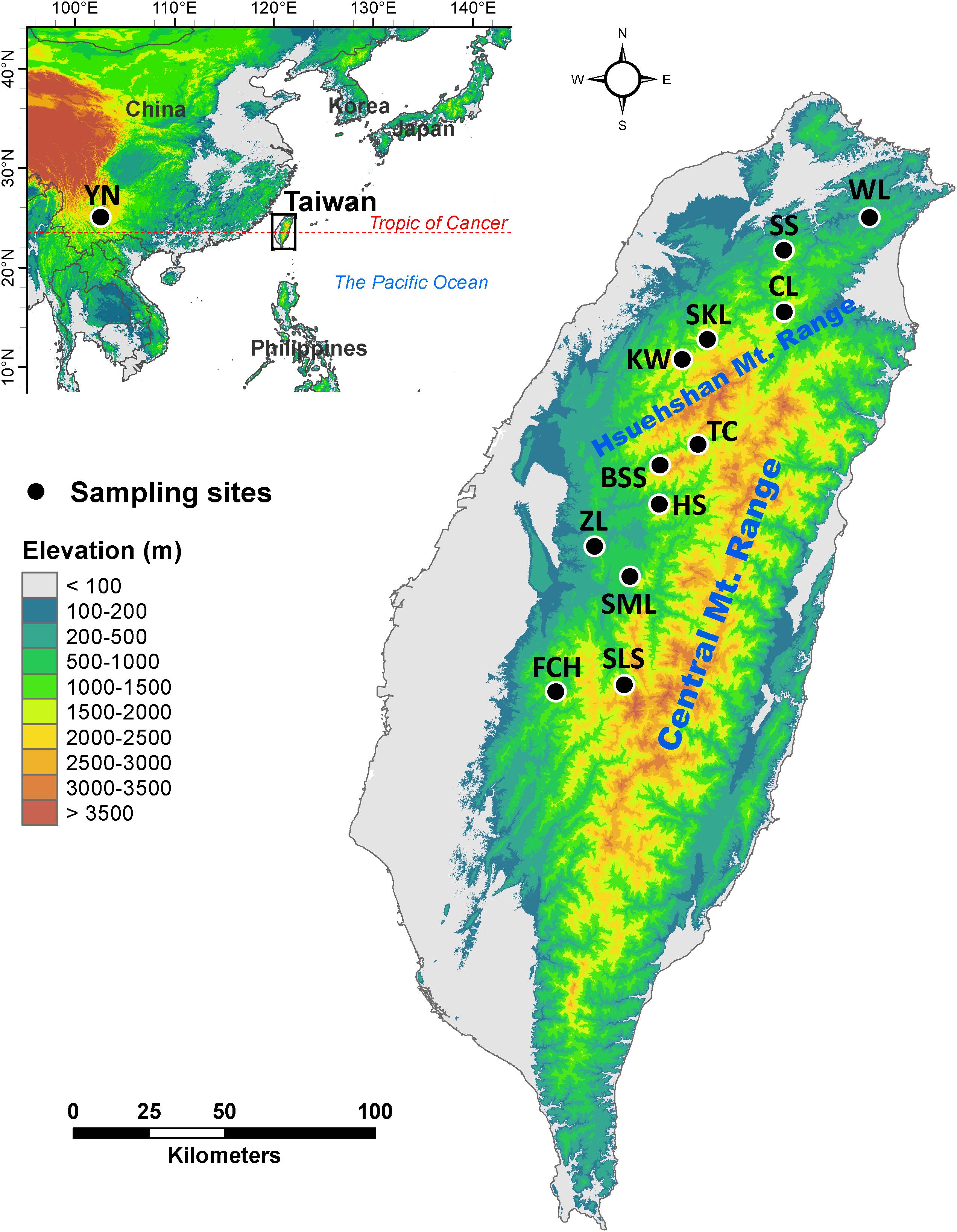
Figure 1. Geographic distribution of the 12 populations of Calocedrus formosana occur in Taiwan. See Table 1 for abbreviations of the 12 populations of C. formosana.
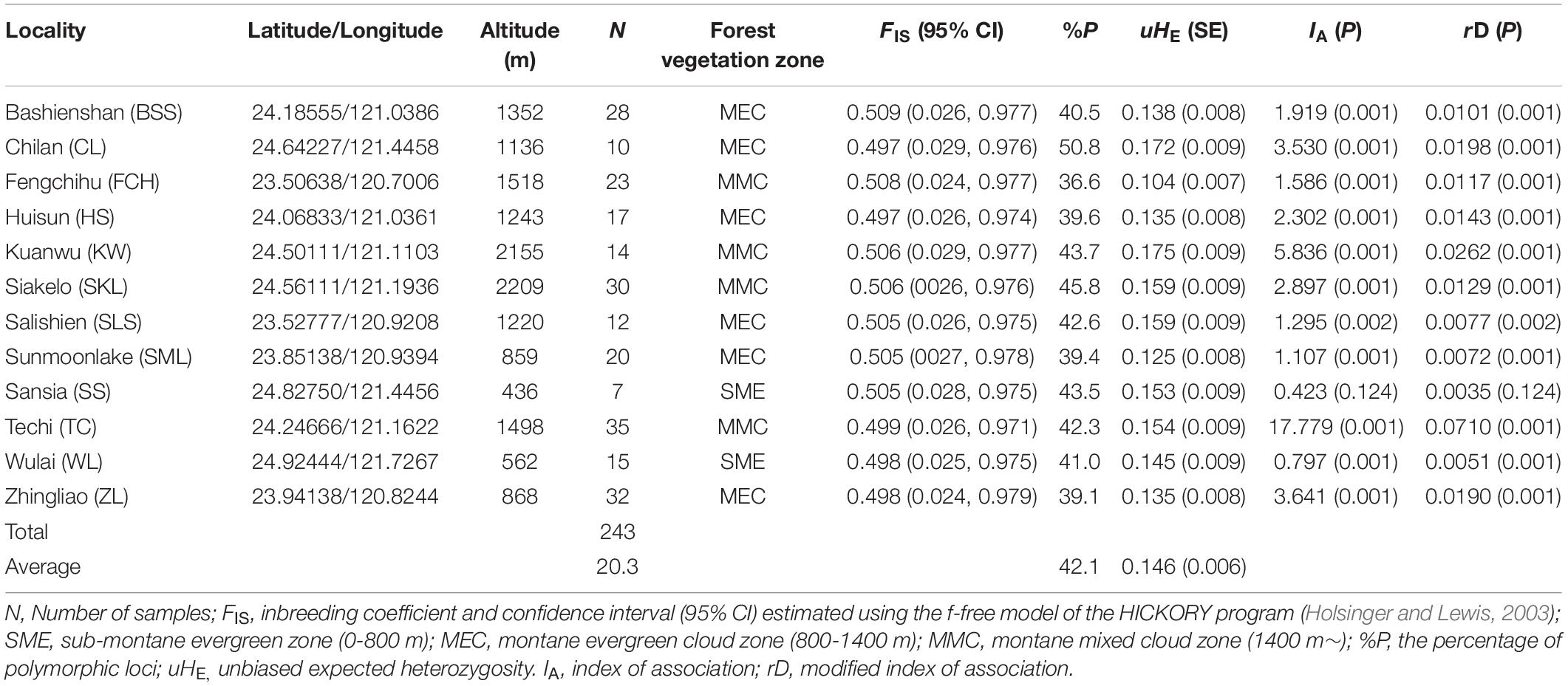
Table 1. Site properties and genetic parameters of the sampled Calocedrus formosana populations.
High elevation populations are typically more vulnerable to environmental change than their low elevation counterparts because of range restriction and dispersal limitations (Savolainen et al., 2007; Allendorf et al., 2010; Hoffmann and Sgrò, 2011). In addition, it was pointed out by Körner (2007) that environmental variables can be classified into two categories: those that are altitude-related, such as temperature; and those that are generally non-altitude-related, such as relative humidity (RH) and sunshine hours (SunH). Therefore, both altitude-related and generally non-altitude related environmental variables may play roles in driving population adaptive divergence. Since the exclusive habitats of C. formosana may be reduced or even disappear in view of global climate change, its unique distribution from low to high elevations makes it useful for investigating the role of elevation on genetic divergence in association with environmental conditions. Information obtained in this study can be useful in the future assisted migration program of C. formosana. We surveyed AFLP variation of 243 samples from 12 populations of C. formosana to examine the role of gene flow on the pattern of population genetic diversity and to test environmentally driven local adaptation in C. formosana populations. Our goals in the present study were to (i) assess whether there is a pattern of genetic diversity along elevation across forest vegetation zones; (ii) test the effect of environment relative to geography on adaptive genetic divergence; and (iii) investigate whether there are low- and high-elevation adaptive genetic loci with high frequencies that are likely to play roles in local adaptation.
Materials and Methods
Sampling and Genotyping
We collected fresh leaf samples of 243 C. formosana individuals from 12 populations distributed in Taiwan (Figure 1 and Table 1). Total DNA was extracted from ground-up leaf powder according to a modified cetyltrimethyl ammonium bromide (CTAB) procedure (Doyle and Doyle, 1987). Ethanol precipitated DNA was washed with 70% ethanol, dissolved in 200 μL TE buffer (pH 8.0) and stored at −20°C until needed. The DNA concentration was determined for each sample using the NanoDrop spectrophotometer (NanoDrop Technology, Wilmington, DE, United States). We quantified genetic variation using AFLP (Vos et al., 1995). Digestion of total genomic DNA (100 ng) was performed using 2 U EcoRI and 2 U MseI (New England Biolabs, Ipswich, MA, United States) and digested DNA products were added to a 10-μl reaction mixture for ligation at 22°C for 1 h. The ligation reaction mixture contains 5 μM of the EcoRI adaptor, 50 μM of the MseI adaptor, and 0.25 U T4 DNA ligase (Real Biotech, Taipei, Taiwan). 1 μl diluted digested samples (1:9 dilution with water) was used as a template to perform pre-selective amplification. Pre-selective amplification was performed in a 10-μl volume containing 1 × PCR buffer (25 mM KCl, 10 mM Tris-HCL, 1.5 mM MgCl2, and 0.1% Triton X-100), 100 nM each of the EcoRI (E00: 5′-GACTGCGTACCAATTC-3′) and MseI (M00: 5′-GATGAGTCCTGAGTAA-3′) primers, 0.25 mM dNTPs, and 1 U Taq DNA polymerase (Zymeset Biotech, Taipei, Taiwan). Conditions of the pre-selective amplification were initial holding at 72°C for 2 min and pre-denaturation at 94°C for 3 min, followed by 25 cycles of 30 s at 94°C, 30 s at 56°C, and 1 min at 72°C, with a final 5-min holding at 72°C. Eleven EcoRI-MseI selective primers combinations with sequences of E00 and M00 and additional bases were added at the ends of these primers (Supplementary Table 1). In selective amplification, EcoRI selective primer was labeled with fluorescent dye (6-FAM or HEX). Conditions of selective amplification were a 10-μl volume containing 1 × PCR buffer, 100 nM of the EcoRI selective primer, 100 nM of the MseI selective primer, 0.25 mM dNTPs, 0.75 U Taq DNA polymerase, and 1 μl diluted pre-selective amplified product (1:9 dilution with water). The selective PCR amplification was performed with initial holding at 94°C for 3 min, followed by 13 cycles of 30 s at 94°C, 30 s at 65°C with 0.7°C touchdown per cycle, and 1 min at 72°C, then 23 cycles of 30 s at 94°C, 30 s at 56°C, and 1 min at 72°C, with a final 5-min holding at 72°C. PCR amplified fragments were separated using an ABI 3730XL DNA analyzer and scored with Peak Scanner v.1.0 (Applied Biosystem, Foster City, CA, United States). We scored AFLP fragments with a fluorescent threshold set at 150 units. Peaks of amplified fragments in the range of 150–500 bp separated by less than one nucleotide in a ±0.8 base pair window were scored as the same fragment. We removed markers scored higher than 99% or less than 1% of individuals. Locus genotyping error rate of each primer combination was calculated based on amplification replicates obtained from three samples in each population. Loci with error rate greater than 5% were removed (Bonin et al., 2004). The mean error rate was 4.91% (Supplementary Table 1). The final AFLP dataset was deposited in Supplementary Data Sheet 1.
Genetic Diversity and Clustering
Proportion of polymorphic loci (%P, 95% criterion) and unbiased expected heterozygosity (uHE) within a population (Nei, 1987) were calculated using AFLP-SURV v.1.0 (Vekemans et al., 2002) based on allele frequencies estimated assuming Hardy-Weinberg equilibrium with non-uniform prior distribution (Zhivotovsky, 1999). Per locus uHE was calculated using ARLEQUIN v.6.0 (Excoffier and Lischer, 2010). Index of association (IA) (Brown et al., 1980) and modified index of association (rD) (Agapow and Burt, 2001), representing multilocus linkage disequilibrium (LD), were calculated using the ia function of R poppr package v.2.8.5 (Kamvar et al., 2015) in the R environment (R Development Core Team, 2018), and significant departure from zero was tested with 999 permutations. The f-free model of a Bayesian approach for dominant marker implemented in HICKORY (Holsinger and Lewis, 2003) was used to estimate inbreeding coefficient (FIS). Assessment of significant difference of mean uHE per locus between populations was performed using a linear mixed model (LMM), based on reduced maximum likelihood estimation, with population as a fixed effect and locus as a random effect using the lmer function of R lme4 package v.1.1-21 (Bates et al., 2015). Significance was assessed based on type II Wald χ2 test using the Anova function of R car package v.3.0-6 (Fox and Weisberg, 2011) with the Tukey method to maintain α = 0.05 using the lsmeans function of R emmeans package v.1.4.3 (Lenth, 2018).
Sparse non-negative factorization (sNMF) algorithm (Frichot and Francois, 2015) and discriminant analysis of principal components (DAPC) (Jombart et al., 2010) were used to assess genetic homogeneous groups of C. formosana individuals. We assessed individual assignments with K = 1–12 based on least-squares optimization using the snmf function of R LEA package v.3.0.0 (Frichot and Francois, 2015). In snmf, the regularization parameter, iterations, and repetitions in snmf were set to 100, 200, and 10, respectively, and other arguments set to defaults. In DAPC, principal component analysis was performed and followed by a discriminant analysis that maximize variance between groups using the find.clusters and dapc functions of R adegenet package v.2.1.2 (Jombart and Ahmed, 2011). The best K in LEA and DAPC was, respectively, evaluated with the mean of minimal cross-entropy (CE) and the Bayesian information criterion (BIC).
Environmental Heterogeneity
We acquired 34 environmental variables and assigned to three categories including 19 bioclimatic, three topological, and 12 ecological variables. Nineteen bioclimatic variables, constituting weather station-based temperature and precipitation information, for sample sites at 30-s spatial resolution (∼1 km) were downloaded from the WorldClim v.1.4 (Hijmans et al., 2005). Topographic variables at 30-m resolution, including aspect, elevation, and slope, were obtained from Aster Global Digital Elevation Map1. Ecological factors obtained were normalized difference vegetation index (NDVI) and enhanced vegetation index (EVI) derived from moderate resolution imaging spectroradiometer (MODIS) dataset MOD13A2 (1 km resolution) and leaf area index (LAI) and fraction of absorbed photosynthetically active radiation (fPAR) derived from a MOD15A2 dataset (500 m resolution). These MODIS datasets were acquired from Land Process Distributed Active Archive Center2 during 2001–2018, and monthly mean values computed using a maximum-value composite procedure (Huete et al., 2002). The annual total potential evapotranspiration (PET) was also included as an ecological variable and calculated based on a MOD16A3 dataset (500 m resolution). Monthly mean values of the other five ecological variables, including RH, cloud cover (CLO), SunH, number of rainfall days per year (RainD), and mean wind speed (WSmean), were calculated with data obtained from the Data Bank for Atmospheric & Hydrologic Research (3 recorded in 1990–2018) at spatial resolution of 1 km using a universal spherical model of the Kriging method in ArcGIS (Chang et al., 2014). Soil pH values of sample sites were obtained based on an island-wide soil investigation (n = 1150) conducted in 1969–1986 obtained from the Agriculture and Food Agency of Taiwan (Chang et al., 2009). Annual moisture index (Thornthwaite, 1948) was calculated based on annual potential evapotranspiration derived from annual mean temperature and annual precipitation.
We used the cor function of R to calculate correlation coefficient (r) between environmental variables. The vif function of R package usdm v.1.1-18 (Naimi et al., 2014) was used to calculate variance inflation factor (VIF) of environmental variables for each environmental category (bioclimate, ecology, and topology) separately. Environmental variables within each category with VIF < 5 and which not strongly correlated with other variables (|r| < 0.8) were retained. Fourteen environmental variables retained were: BIO1 (annual mean temperature), BIO7 (annual temperature range), BIO12 (annual precipitation), and BIO18 (precipitation of the warmest quarter) of bioclimatic category; aspect, elevation, and slope of topological category; and fPAR, NDVI, RH, RainD, soil pH, sunH, and WSmean of ecological category (Supplementary Table 2). The matrix of pairwise correlation coefficient between these environmental variables was used to depict correlation plot using the corrplot function of R package corrplot v.0.84 (Wei and Simko, 2017).
To assess environmental differences among sample sites and among sample sites of the three genetic clusters (see section “Results”), Euclidean distance matrix was generated using the dist function of R for the 14 retained environmental variables and used in a permutational multivariate analysis of variance (PERMANOVA) using adonis function of R package vegan v.2.5-6 (Oksanen et al., 2017). Pairwise comparison was performed using the pairwise.perm.manova function of R package RVAideMemoire v.0.9-74 (Herve, 2018). Significance of pairwise comparisons was tested with 999 permutations and a false discovery rate (FDR) of 5%.
Test for FST Outliers
Two FST-based methods (BAYESCAN and DFDIST) were used to identify FST outliers indicating signature of selection across populations. BAYESCAN v.2.1 (Foll and Gaggiotti, 2008) uses a reversible-jump Markov chain Monte Carlo algorithm to estimate the ratio of posterior probabilities of selection over neutrality [the posterior odds (PO)] using hierarchical Bayesian method. Two hundred pilot runs of 50,000 iterations were performed followed by a sample size of 50,000 with thinning interval of 20 among 106 iterations in BAYESCAN analysis. A logarithmic scale of log10PO > 0.5, of log10PO > 1.0, of log10PO > 1.5, and of log10PO > 2 was, respectively, defined as substantial, strong, very strong, and decisive evidence for selection over neutrality according to Jeffreys (1961) and Foll (2012). In the present study, we considered a locus with log10PO > 2 as a potential selective outlier.
The Beaumont and Nichols model, modified for dominant marker, implemented in DFDIST (Beaumont and Nichols, 1996) was used to estimate a distribution of observed FST (Weir and Cockerham, 1984) versus uHE (Zhivotovsky, 1999). Loci that may be under selection were identified by comparing to a simulated neutral distribution. Parameters include critical frequency = 0.99; Zhivotovsky parameters = 0.25; trimmed mean FST = 0.3 (excluding 30% of highest and 30% of lowest FST values); smoothing proportion = 0.04; 500,000 resamplings; critical P = 0.05, and target average θ (level of differentiation) = 0.099575 were used for running DFDIST. In DFDIST, significant P values of FST outliers were evaluated at the 99% confidence level with 5% FDR.
Test for Associations of Genetic Loci With Environmental Variables
Samβada v.0.8.3 (Stucki et al., 2017) and latent factor mixed model (LFMM) implemented in the lfmm function of R LEA package (Frichot et al., 2013) were used to assess the associations of all the genetic loci with environmental variables. Samβada employs a multiple univariate logistic regression approach to assess the significant correlations of allele frequencies with the values of environmental variables. Both Wald and G scores with an FDR cutoff of 0.01 were applied to assess the significant fit of model with environmental variables compared to null model without environmental variables. LFMM uses a hierarchical Bayesian mixed model considering background level of population structure, latent factors (K), as a random effect due to demographic history and IBD pattern. Genetic data was used as a fixed effect in a testing procedure based on Z-scores. The number of latent factors, K, was set to 3 based on the results of LEA and DAPC analyses (see section “Results”). Five LFMM runs for each value of K with 10,000 iterations of the Gibbs sampling algorithm and a burn-in period of 5,000 cycles were performed. Z-scores of five independent runs were combined using Fisher-Stouffer method (Brown, 1975), and the resulting P-values were adjusted using the genomic inflation factor (λ). An FDR correction of 1% was further used in P-value adjustment using the q-Value function of R q-value package v.2.20.0 (Storey et al., 2019). AFLP loci recognized as outliers potentially evolved under selection were those FST outliers detected either by BAYESCAN or by DFDIST and found to be strongly associated with environmental variables.
We used a Bayesian logistic regression analysis implemented in the stan_glm function of R rstanarm package v.2.19.2 (Goodrich et al., 2018) to further verify the associations of FST outliers detected by BAYESCAN and DFDIST with environmental variables. Student’s t distribution with mean zero and seven degrees of freedom were used as the weakly informative priors, and the scale of the prior distribution was 10 for the intercept and 2.5 for the predictors. All stan_glm models were run with four chains for 2000 warm-up and 2000 sampling steps. The posterior_interval function of R rstanarm package was employed to estimate 95%, 99%, and 99.5% credible intervals for determination of significant correlations of FST outliers with environmental variables.
Genetic Differentiation
Both the total and the outlier data were used in analysis of molecular variance (AMOVA). AMOVA was used to estimate the levels of population genetic differentiation at the hierarchical levels of geographic areas north and south of the HMR, genetic clusters (see section “Results”), and sample sites using the poppr.amova function of R package poppr, and significance tested using the randtest function of R package ade4 v.1.7-13 (Dray and Dufour, 2007) with 9,999 permutations. Pairwise FST was computed using ARLEQUIN based on the total data and significance tested with 10,000 permutations.
Mantel Test, Variation Partitioning, and Forward Selection
Mantel test was used to analyze the correlations of the AFLP Euclidean distance matrix with the Euclidean distance matrix of geography (latitude and longitude) and with the matrix of elevational difference using the mantel function of R vegan package. The retained environmental variables in the three environmental categories (bioclimatic, ecological, and topological categories) were analyzed separately using redundancy analysis (RDA) to assess the relative contribution of environmental variables in each category explaining the outlier AFLP variation using the varpart function of R package vegan, and significance tested using the anova.cca function with 999 permutations. Four fractions of the total outlier variation were partitioned: pure environmental variables (fraction [a]), geographically structured environmental variables (fraction [b]), pure geographic variables (fraction [c]), and residual effects (fraction [d]) (Borcard et al., 1992; Borcard and Legendre, 2002). The amount of the outlier variation explained in each fraction was determined based on adjusted R2 values (Peres-Neto et al., 2006). Longitude and latitude of sample sites were used as geographic variables in the analysis. The double-stopping criterion (Blanchet et al., 2008) of the forward.sel function of R adespatial package v.0.3-7 (Dray et al., 2019) was used to estimate the most important environmental variables explaining the outlier genetic variation and significance determined using 999 permutations.
Results
Diversity
We obtained 437 AFLP (mean ± SD: 39.7 ± 12.0) loci using 11 selective amplification primer combinations (Supplementary Table 1). The average percentage of polymorphism was 42.1 (ranged from 36.6 for the population FCH to 50.8 for the population CL) (Table 1). The average level of uHE was 0.146 and ranged between 0.104 (population FCH) and 0.175 (population KW). No positive correlation between population uHE and sample size was found based on Spearman’s rank correlation test (ρ = -0.371, P = 0.237). The measures of multilocus LD, IA and rD, showed significant departure from random association between AFLP loci for all populations except the population SS (Table 1). Moreover, population FIS estimated using the f-free model of HICKORY ranged between 0.497 and 0.509.
Within C. formosana, LMM analysis showed the level of mean uHE per locus was significantly different among populations (χ2 = 164.24, P < 0.0001). Significant difference was also found in many pairwise population comparisons (Supplementary Table 3), in which paired populations in comparisons were found not only located in the same, but also in different forest vegetation zones.
Genetic Structure
The mean of minimal CE was minimized after K = 4 in LEA analysis (Supplementary Figure 1A) and the BIC in DAPC analysis was minimized at K = 5. (Supplementary Figure 1B). However, three genetically homogeneous groups were most reasonably displayed by both LEA and DAPC (Figures 2, 3). The amount of genetic variation explained by the first two linear discriminants was, 50.61% and 31.63%, respectively (Figure 3). The first cluster contains populations WL, SS, CL, SKL, KW, and SLS. The second cluster contains populations TC, BSS, and HS. Populations SML, FCH, and ZL were included in the third genetic cluster. Using the total data, AMOVA revealed significant differentiation at all hierarchical structuring levels analyzed between populations (ΦST = 0.1402, P < 0.001), between populations of different genetic clusters (ΦST = 0.1283, P < 0.001), and between north and south of the HMR (ΦST = 0.0967, P < 0.001) (Table 2). However, the level of population differentiation between north and south of the HMR was relatively low compared to across population differentiation, albeit significant. The average pairwise FST was 0.1327 based on the total data (Supplementary Table 4).
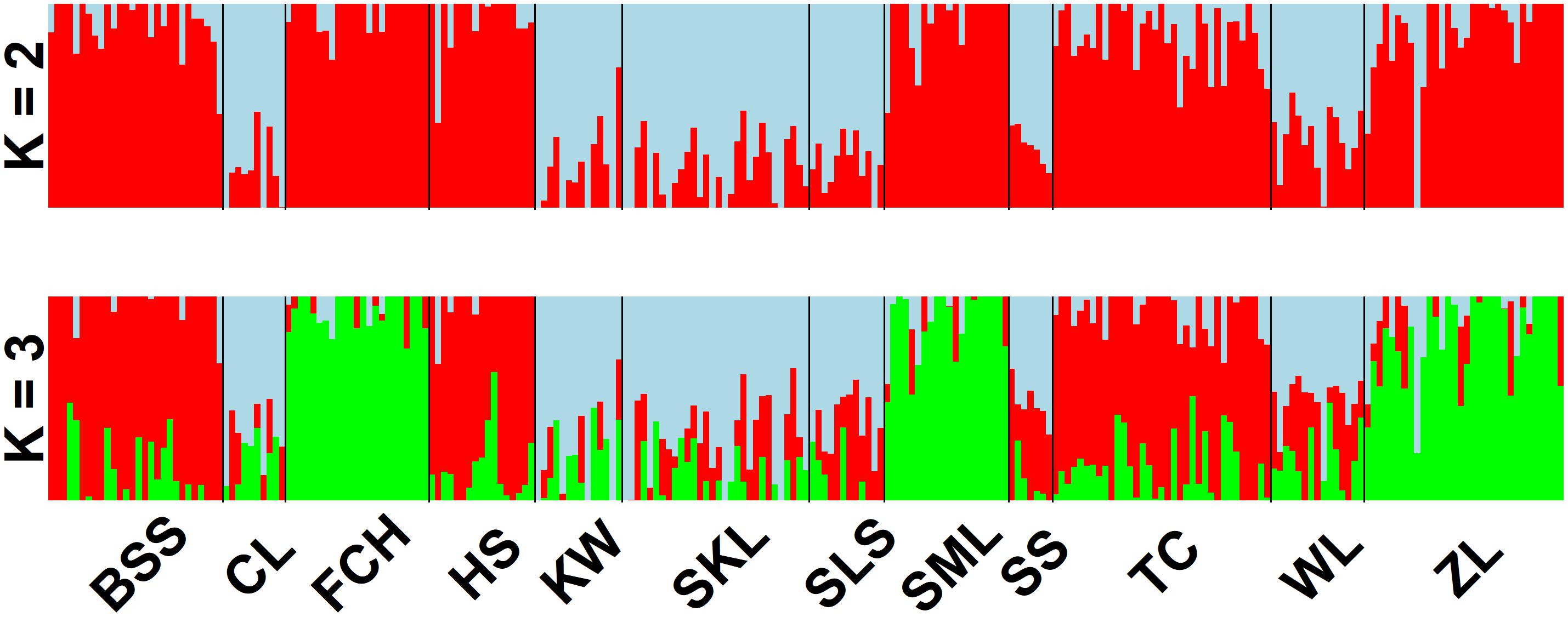
Figure 2. Individual assignments of 243 individuals from 12 populations of Calocedrus formosana analyzed using LEA. The clustering scenarios for K = 2–3 were displayed.
Figure 3. Clustering results analyzed using discriminant analysis of principal components (DAPC) for the 243 individuals from 12 populations of Calocedrus formosana.
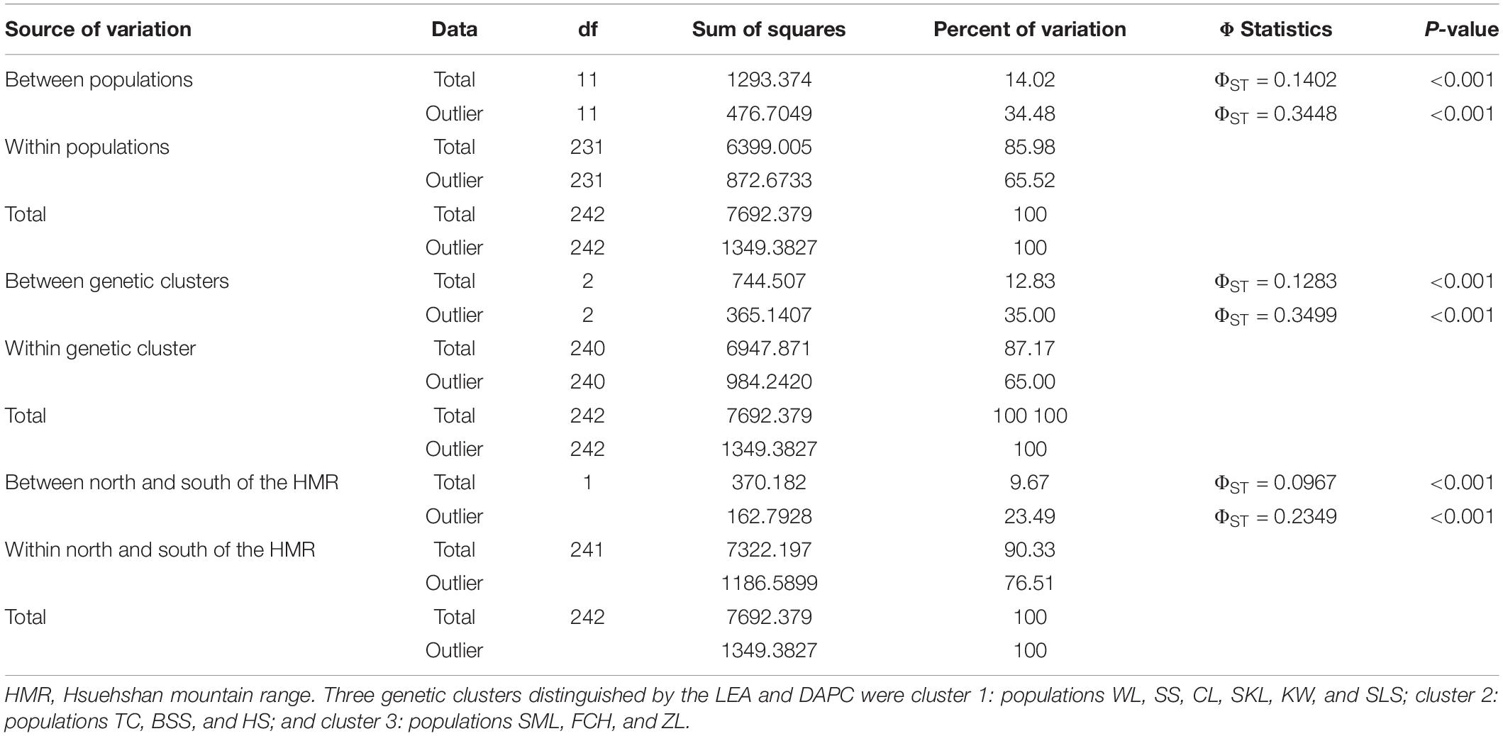
Table 2. Summary of the analysis of molecular variance (AMOVA) based on the total and the outlier genetic variations.
Potential Selective Outliers and Outlier Genetic Differentiation
BAYESCAN identified 26 loci as potential selective outliers (Table 3). Nine loci were identified as potential outliers by DFDIST; however, none of these loci remained significant after FDR correction. All 26 outliers identified by BAYESCAN were found to be strongly associated with environmental variables assessed using Samβada and LFMM (Table 3). The corresponding Z-scores and q values of candidate outlier loci identified using LFMM were summarized in Supplementary Table 5. The associations of potential selective outlier loci with more than one environmental variable were commonly observed, and therefore, Bayesian logistic regression was further used to assess the relationships between those outliers with environmental variables. Analysis using Bayesian logistic regression confirmed the associations of outlier loci with more than one variable within each environmental category (i.e., bioclimate, ecology, and topology) (Table 3).
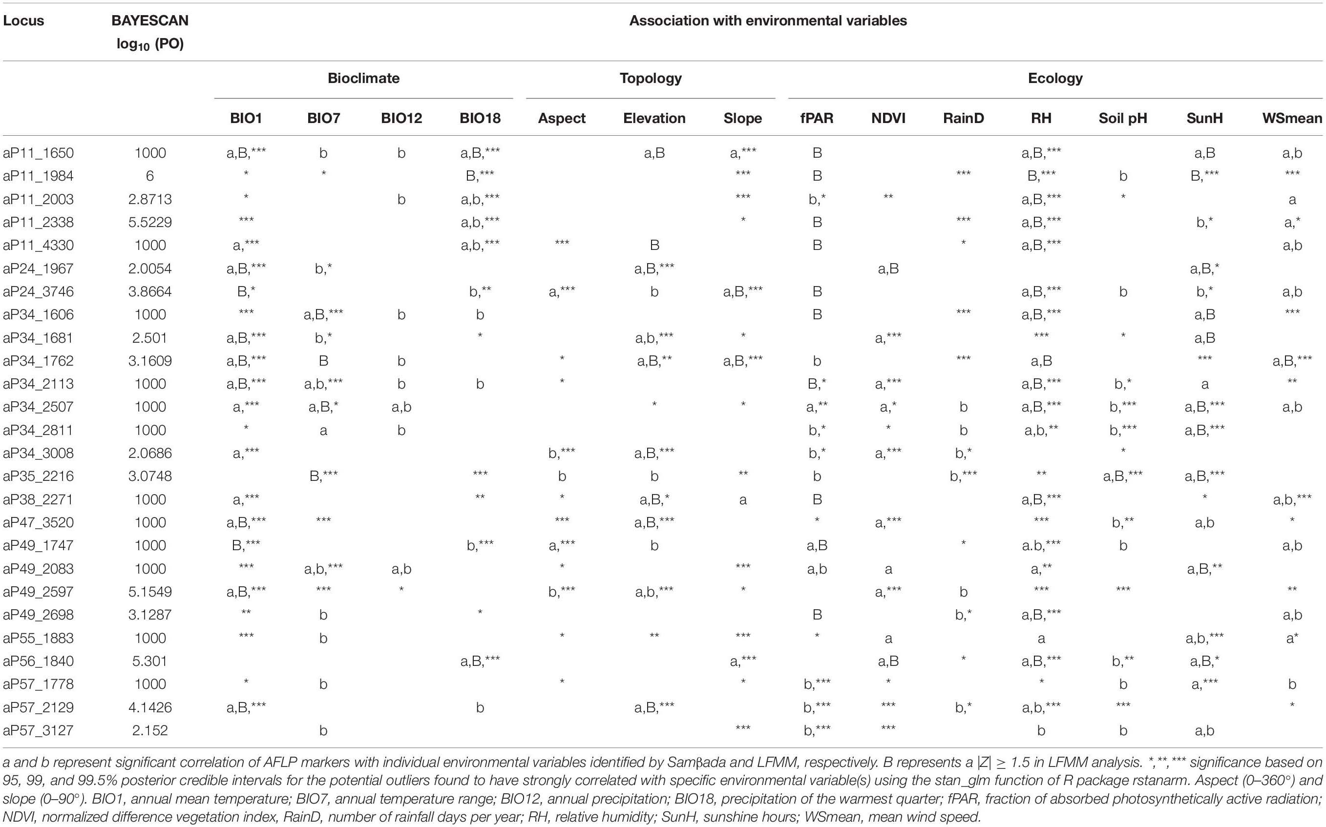
Table 3. Potential outliers identified by BAYESCAN and DFDIST associated with environmental variables.
Allele frequencies of the outlier loci across populations arranged altitudinally were depicted in Figure 4A. The most prominent outlier AFLP loci with high frequencies uniquely at low elevations were aP11_2338 (population SS) and aP34_1606 (population SS). At high elevations, aP57_1778 (population KW) was the most prominent outlier AFLP locus. Additionally, there were also outlier AFLP loci, e.g., aP34_3008 (population SLS), aP35_2216 (population HS), and aP49_2698 (population SLS), found to have high frequencies at middle elevations between 800 and 1400 m in the montane evergreen cloud zone. Medium frequency outlier AFLP loci were also commonly observed at different elevational ranges corresponding to different forest vegetation zones.
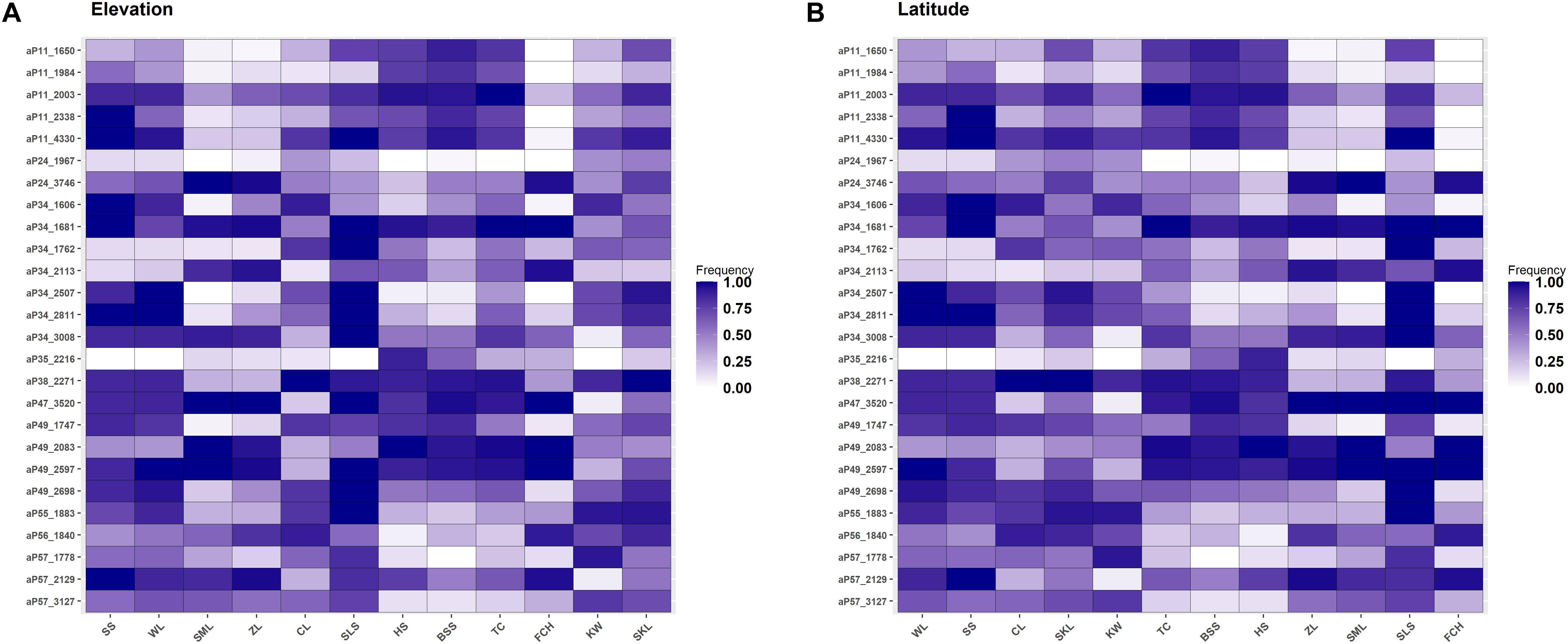
Figure 4. Heatmap of allele frequencies of the 34 outlier loci identified. The sequence of populations was arranged according to (A) elevation or (B) latitude.
Genetic differentiation analyzed using AMOVA, based on the outlier data, showed significant outlier genetic differentiation between populations (ΦST = 0.3448, P < 0.001; Table 2), between populations of the three genetic clusters (ΦST = 0.3499, P < 0.001), and between populations north and south of the HMR (ΦST = 0.2349, P < 0.001).
Outlier Genetic Variation Explained by Environment and Geography and the Most Important Environmental Variables Associated With the Outlier Variation
The correlation between the 14 retained environmental variables was depicted in Supplementary Figure 2. Although PERMANOVA revealed no environmental difference across populations (P = 1), significant environmental differences between sample sites and between sample sites of different vegetation zones were found (Supplementary Table 6). Additionally, environmental heterogeneity was found when compared among the sample sites grouped into three genetic clusters (F = 23.01, R2 = 0.1609, P = 0.001). Mantel test revealed significant IBD based on the total and the outlier data (total data: Mantel R2 = 0.185, P = 0.0001; outlier data: Mantel R2 = 0.348, P = 0.0001). Total explainable outlier genetic variation was 18.52%, 30.09%, and 19.64%, respectively, for bioclimatic, ecological, and topological variables analyzed separately (Table 4). In all three environmental categories, the amount of explained variation was relatively small as compared to the amount of unexplained variation (fraction [d]). Based on the outlier genetic data and analyzed the three environmental categories separately, pure ecological factor was found to be the most influential environmental variables contributing to the outlier genetic variation (18.75%) in contrast to pure bioclimatic (7.18%) and pure topological (8.30%) factors. Within bioclimatic and within ecological category, pure environmental factor explained much larger proportion of the outlier genetic variation than those explained by pure geography (7.18% vs. 4.26%; 18.75% vs. 4.45%, respectively). However, pure geography (11.84%) explained a larger fraction of the outlier variation than pure topological factors (8.30%) within the topological category. Additionally, outlier genetic variation can also be explained by geographically structured environmental variables in bioclimatic and in ecological category (7.07% and 6.89%, respectively), but no outlier genetic variation was explained by geographically structured environmental variables in topological category.
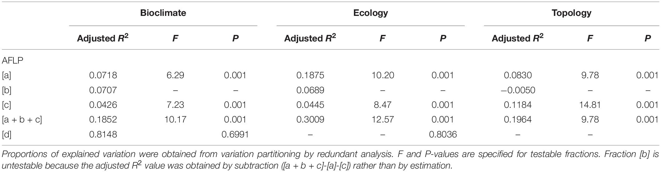
Table 4. The percentage of the outlier genetic variation accounted for by non-geographically structured environmental variables [a], shared (geographically structured) environmental variables [b], pure geographic factors [c], and undetermined component [d] analyzed based on the 14 retained environmental variables in three environmental categories (bioclimate, ecology, and topology).
We assessed the most important variables in each environmental category accounted for the outlier genetic variation using forward selection (Blanchet et al., 2008). The most significant influential environmental variable was annual mean temperature (bioclimate), relative humidity (ecology), and elevation (topology) (adjusted R2 = 5.67%, adjusted R2 = 13.69%, and adjusted R2 = 3.55%, respectively) based on the outlier data (Table 5).
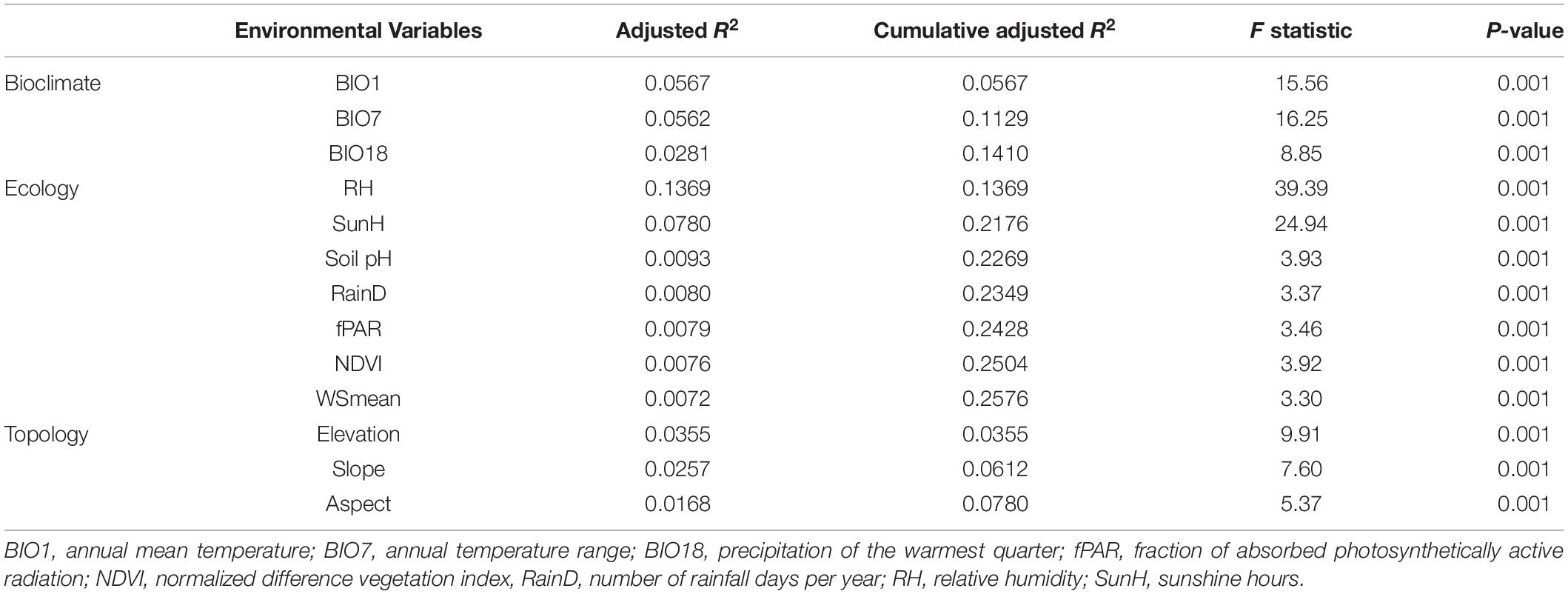
Table 5. Environmental variables selected by a forward selective procedure explaining outlier genetic variation in Calocedrus formosana.
Discussion
Patterns of Diversity and the Roles of Gene Flow and Environments on Population Diversification
Population genetic diversity is the basis for evolution in a species that can result from the balance between gains of new mutations and drift-mediated loss of alleles (Kimura and Crow, 1964; Barrett and Schluter, 2008; Jump et al., 2009). Plants that occupy restricted geographic range are expected to have reduced level of genetic diversity (Hamrick and Godt, 1989; Cole, 2003). However, C. formosana distributed in a wider elevational range lower level of AFLP genetic diversity (average uHE = 0.146) was found compared with other Taiwanese conifers with narrower geographic distributions such as K. davidiana var. formosana (average uHE = 0.233, Fang et al., 2013), C. konishii (uHE = 0.203, Li et al., 2019), and T. cryptomerioides (uHE = 0.236; Li et al., 2018).
Genetic diversity is greater for central than for marginal populations because conditions at the central portion of the range are optimal, but environments at the edges can be stringent (Lesica and Allendorf, 1995; Eckert et al., 2008). Although migration can contribute intra-population genetic diversity (Maruyama, 1970; Nei, 1973; Barrett and Schluter, 2008; Jump et al., 2009), populations located at the outer boundaries of the species’ range genetic drift can be promoted, thereby reducing genetic diversity and increasing differentiation from central populations (Kimura and Crow, 1964; Maruyama, 1970; Nei, 1973; Barrett and Schluter, 2008; Jump et al., 2009). Our results of the level of uHE along elevational gradient in the present study are not consistent with the abundant-center hypothesis and higher levels of uHE can be found in the outer margin (low- and high- elevations) populations compared with that of central populations (c.f. Assis et al., 2013; Figure 1 and Table 2).
The positive FIS and significant multilocus LD can result from bottlenecks because of mating among genetically close individuals within populations (Przeworski, 2002; Wall et al., 2002). Past bottleneck events can effectively cause reduction in sample size, loss of connectivity, increase in genetic drift, and increase in the probability of inbreeding (Reed and Frankham, 2003). The current reproductive mode of inbreeding is evident in C. formosana populations because of significant positive FIS values estimated for all populations and significant departure from random association based on the measures of multilocus LD in all but one of the populations examined (IA and rD, Table 1). The non-random breeding or mating between genetically close relatives of a population could be a general phenomenon in Taiwanese conifers because significant positive FIS and significant departure from random association are also found in other Taiwanese conifers such as C. konishii, K. davidiana var. formosana, and T. cryptomerioides (Fang et al., 2013; Li et al., 2018, 2019). Moreover, the magnitude of loss of alleles might be greater in C. formosana populations compared with the other three Taiwanese conifers. Nonetheless, divergent selection invoked by environmental heterogeneity, resulting in the higher level of population differentiation compared with other Taiwanese conifers (Fang et al., 2013; Li et al., 2018, 2019), might have also contributed to the detection of significant multilocus LD (Kawecki and Ebert, 2004; Nosil et al., 2005; Jump and Peñuelas, 2006).
Efficient migration can be the cause for the low level of differentiation between subdivided populations (Maruyama, 1970; Nei, 1973) and the general realization in conifers is the high rates of effective pollen dispersal, resulting in low population differentiation (Hamrick et al., 1992; Hamrick and Godt, 1996). Relatively higher level of the average pairwise FST was found in C. formosana (=0.1327) based on the total data in the present study (Supplementary Table 4) compared to other Taiwanese conifers such as T. cryptomerioides (average pairwise FST = 0.041, Li et al., 2018), C. konishii (average pairwise FST = 0.102, Li et al., 2019), and K. davidiana var. formosana (average pairwise FST = 0.061, Fang et al., 2013). AMOVA also showed higher level of across population differentiation based on the total data in C. formosana (ΦST = 0.1647) compared to T. cryptomerioides (ΦST = 0.0316, Li et al., 2018), C. konishii (ΦST = 0.0827, Li et al., 2019), and K. davidiana var. formosana (ΦST = 0.0632, Fang et al., 2013) occurring in Taiwan. The higher level of population differentiation in C. formosana might have been caused by a relatively lower rate of gene flow, resulting in larger degree of drift-mediated loss of alleles (Kimura and Crow, 1964; Conner and Hartl, 2004; Barrett and Schluter, 2008; Jump et al., 2009).
Nonetheless, environments may also play roles in shaping population differentiation (Kawecki and Ebert, 2004; Nosil et al., 2005; Jump and Peñuelas, 2006; Holderegger et al., 2008; Jump et al., 2009; Table 2). PERMANOVA revealed differences in environmental conditions between sample sites and between sample sites of different vegetation zones (Supplementary Table 6), suggesting that environmental heterogeneity between sample sites and between sample sites located in different vegetation zones might have played roles in driving population differentiation along elevational gradients. In the present study, Mantel test revealed significant IBD based on the total and the outlier data. Moreover, mountains might not have played a significant role as barriers to gene flow between north and south of the HMR because AMOVA showed a lower level of differentiation based on the total data (ΦST = 0.0967, Table 2) for populations located between these two geographic areas compared to the higher level of across population differentiation (ΦST = 0.1402). The HMR may not act as an effective barrier to gene flow can also be supported by the grouping of population SLS located in the south of the HMR with populations WL, SS, CL, SKL, and KW located in the north of the HMR in the same genetic cluster revealed by the LEA and DAPC analyses (Figures 1, 2).
Evolutionary divergence can occur in the presence of gene flow (Wu, 2001) and the magnitude of migration might have a relationship with the probability of detecting adaptive divergence in these Taiwanese conifers. The number of environmentally dependent selective outliers among the four Taiwanese conifers mentioned might have a positive relationship with the level of population differentiation. The number of environmentally dependent selective outliers out of the total AFLP loci scored are 0/1413 (0%, T. cryptomerioides, Li et al., 2018), 3/465 (0.65%, K. davidiana var. formosana, Fang et al., 2013), 15/482 (3.11%, C. konishii, Li et al., 2019), and 26/483 (5.95%, C. formosana, Table 3). It is worthy to note that more FST outliers were detected in the present study even a more stringent criterion (log10(PO) > 2) for outlier identification was employed in BAYESCAN as compared to the criterion of log10(PO) > 0.5 used in the other three previous studies.
In general, we can summarize a pattern of lower level of genetic diversity along with the higher level of genetic differentiation for Taiwanese conifers including C. konishii, K. davidiana var. formosana, T. cryptomerioides, and C. formosana. The relationship of higher number of environmentally dependent selective outliers detected with higher levels of genetic differentiation in these conifers suggests that gene flow among environmentally distinct populations can be effective in homogenizing locally adapted alleles and dampened local adaptation driven by natural selection (Kirkpatrick and Barton, 1997; Lenormand, 2002; Sexton et al., 2014).
Ecological Factors Played the Most Prominent Roles in Driving Adaptive Evolution
Geography and environment can both be effective barriers to gene flow between populations (Hahn et al., 2012; Wang et al., 2013; Sexton et al., 2014; Reis et al., 2015; Antonelli, 2017; Feijó et al., 2019). These factors are not mutually exclusive and they are closely related directly or indirectly influencing the process of dispersal (Wang et al., 2013; Huang et al., 2016), and we are expecting to find both geography and environment explaining the outlier genetic variation to a certain degree. Variation partitioning controlling for geographic distance revealed significant amounts of the outlier genetic variation explained by variables in all three environmental categories (Table 4). Interestingly, ecological factors explained a relatively larger amount of the outlier variation compared to the amount of the outlier variation explained by bioclimatic factors and explained by topological factors in separate analyses. Various environmental conditions can lead to fitness-related adaptation to local conditions (Storz, 2010), reflecting in the level of differentiation as revealed by AMOVA based on environmentally dependent outlier data (ΦST = 0.3448, Table 2). Additionally, forward selection found that the most important variable in three environmental categories explaining the outlier genetic variation, respectively, was annual mean temperature, relative humidity, and elevation (Table 5). However, environmental variables in three environmental categories explaining more than 5% of the outlier genetic variation were annual mean temperature and annual temperature range (bioclimatic variable, adjusted R2 = 0.0567 and adjusted R2 = 0.0562, respectively) and relative humidity and sunshine hours (ecological variable, adjusted R2 = 0.1369 and adjusted R2 = 0.0780, respectively).
Temperature can play a significant role in shaping genetic divergence and enhancing speciation rate (Allen et al., 2006; Strasburg et al., 2012). It is commonly found that temperature plays a prominent role as a selective driver for adaptive divergence in various plant species (Manel et al., 2010, 2012; Bothwell et al., 2013). Temperature was also found to be one of critical environmental variables, in plant species occurring in Taiwan, strongly associated with genetic variation analyzed using expressed sequence tag simple sequence repeats (EST-SSRs) (Hsieh et al., 2013) and AFLP and methylation-sensitive amplification polymorphism (Huang et al., 2015b) in Rhododendron oldhamii. Temperature was also found to be strongly associated with AFLP variation in K. davidiana var. formosana (Fang et al., 2013), in Salix fulvopubescens (Huang et al., 2015a) and in C. konishii (Li et al., 2019). Association of single nucleotide polymorphism with temperature was also found in K. davidiana var. formosana (Shih et al., 2018). In C. formosana, annual mean temperature and annual temperature range might have played a crucial, but minor role involved in adaptive divergence (adjusted R2 = 0.0567 and adjusted R2 = 0.0562, Table 5) compared to ecological factors such as relative humidity (adjusted R2 = 0.1369, P = 0.001) and sunshine hours (adjusted R2 = 0.0780). Using a Mantel test, significant isolation by elevation was found based on the total (Mantel R2 = 0.257, P = 0.001) and the outlier (Mantel R2 = 0.289, P = 0.001) genetic data. However, elevational difference in meters cannot be the causal factor in driving population adaptive divergence (Körner, 2007) and elevation in topological category explained a relatively smaller fraction of the outlier variation (adjusted R2 = 0.0355) compared with annual mean temperature and annual temperature range in bioclimatic category, and relative humidity and sunshine hours in ecological category (Table 5). It is likely that adaptive divergence in C. formosana could have been invoked by the combination of environmental variables, particularly the combinatorial effect of altitude-related temperature and generally non-altitude-related relative humidity and sunshine hours. Relative humidity and sunshine hours significantly explaining the outlier genetic variation (cumulative adjusted R2 = 0.2176, Table 5) could be the most important environmental factors driving adaptive genetic variation in C. formosana. For plant species occurring in Taiwan, EST-SSR and AFLP variations were found to be strongly associated with relative humidity and sunshine hours in R. oldhamii (Hsieh et al., 2013). Relative humidity was also found to be associated with AFLP variation in K. davidiana var. formosana (Fang et al., 2013).
Variation partitioning also revealed significant amounts of the outlier genetic variation explained by geographically structured environmental conditions in bioclimatic and ecological environmental categories (Table 4), indicating that spatially shaped latent environmental variables also might have played an important role invoking adaptive genetic divergence in C. formosana (c.f. Nakazato et al., 2007; Huang et al., 2015a,b, 2016; Li et al., 2018, 2019).
Although aspect and slope might have only played minor roles in shaping genetic variation in C. formosana in the present study (Table 5), these two topological factors were found to be critical in shaping genetic variation of other plant species (e.g., Manel et al., 2003; Huang et al., 2015a; Shih et al., 2018). Aspect and slope can be important in influencing habitat microclimate (Hörsch, 2003; Bennie et al., 2008; Brousseau et al., 2015) and contributed to intra- and inter-species adaptive divergence (Manel et al., 2010, 2012; Nakazato et al., 2010; Monahan et al., 2012; Bothwell et al., 2013; Brousseau et al., 2015). Habitat-associated microclimate is also found to have a relationship with elevation (Clinton, 2003; Bell et al., 2014; Sunday et al., 2014). A single environmental factor is not always sufficient to explain local vegetation penology (Hwang et al., 2011) and it is probable that elevation, slope, and aspect in combination can have influence on tree structure and growth (Turner et al., 2001; Montoya-Pfeiffer et al., 2016; Hu et al., 2018), and increase the effects of IBE contributing to the geographic patterns of climatically and ecologically structured genetic variation.
Adaptive Evolution at Elevational Margin Populations
The amount of genetic diversity, the strength of natural selection, and the extent of gene flow can all influence the probability of the occurrence of local adaptation (Hoffmann and Sgrò, 2011). Local adaptation can occur in association with conditions in different parts of a species’ distribution range and adaptive potential at elevational edges is particularly important for species’ contraction and expansion following climate change (Byars et al., 2007; Leimu and Fischer, 2008; Hereford, 2009; Chen et al., 2014; Rumpf et al., 2019; Zhang et al., 2019). However, central populations can also be vulnerable in the face of global climate change (Bennett et al., 2015). Our results of finding high frequency outlier loci at high- and low-elevations (Figure 4A) are in consistent with findings of evolutionary adaptation occur in leading- and trailing-edge populations of species shifting their ranges because of warming (Ackerly, 2003; Hampe and Petit, 2005; Thuiller et al., 2008; Chen et al., 2014; Rödin-Mörch et al., 2019). Additionally, outlier loci beginning to accumulate their frequencies at different elevations were also observed, suggestive of an ongoing process of outliers accumulating frequencies as selective pressures persist at local scales. In contrast, we did not find high frequency outlier loci specifically at the populations of extreme latitudinal ends of C. formosana distribution range (Figure 4B).
Biogeographical as well as ecological factors can affect the level of diversity within and among populations (Pérez de Paz and Caujapé-Castells, 2013). Forest upward migration of 1,500 to 1,600 m in Taiwan since the last glacial maximum has been reported (Liew and Chung, 2001) and mountain plants experienced an upward migration of ca. 3.6 m per year during the last century has also been reported (Jump et al., 2012). Nonetheless, it is common that species and genera continued to grow at the same latitude even though suitable habitats would have been reduced when forest species distributions shifted upward to a different range of elevations in response to postglacial climatic warming (Tsukada, 1966; Liew and Chung, 2001). It is probable that high elevation populations (populations KW and SKL) are recently colonized because of distribution range shifting upward, and they encountered ecological discontinuity invoking the evolution of environmentally associated genetic variation underlying local adaptation. Moreover, trailing-edge populations persisted at low elevations environmentally dependent genetic variation can also be evoked (Byars et al., 2007; Leimu and Fischer, 2008; Hereford, 2009; Chen et al., 2014; Zhang et al., 2019).
Conclusion
For plants with limited dispersal capabilities, global climate change may manifest the risk of extinction because of loss of the unique genetic diversity at elevational margin populations. Here, our results showed no pattern of population genetic diversity in consistent with the abundant central hypothesis. Relatively lower level of genetic diversity and higher level of genetic divergence were found compared with other Taiwanese coniferous species such as C. konishii, K. davidiana var. formosana, and T. cryptomerioides. Moreover, strong migration may also inflict the break-up of locally adapted gene complex. Nonetheless, increased divergence associated with environmental variables at the edge populations of plant species shifting their range altitudinally may provide insights into the adaptive evolution of species. A higher portion of genetic loci was found to be environmentally dependent in C. formosana compared with the three other Taiwanese conifers. Additionally, our results revealed the associations of high frequency outlier loci with environmental variables, including altitude-related annual mean temperature and annual temperature range and generally non-altitude-related relative humidity and sunshine hours at elevational margin populations. Relative humidity and sunshine hours generally not altitude specific could have been the major ecological drivers invoked adaptive divergence in C. formosana. Results of this study and the previous studies provide insights into the interplay of gene flow and environments in shaping population genetic divergence in Taiwanese conifers.
Data Availability Statement
The AFLP data used in this study is included in the article/ Supplementary Data Sheet 1.
Author Contributions
S-YH proposed, funded, and designed the research. W-MC, Y-CC, and S-YH collected the samples. W-MC, C-TC, and S-YH performed the research. S-YH and W-MC wrote the manuscript. All authors analyzed the data and read and approved the final manuscript.
Funding
This work was funded by the Taiwan Ministry of Science and Technology under grant number of MOST 106-2313-B-003- 001-MY3.
Disclaimer
Frontiers Media SA remains neutral with regard to jurisdictional claims in published maps and institutional affiliations.
Conflict of Interest
The authors declare that the research was conducted in the absence of any commercial or financial relationships that could be construed as a potential conflict of interest.
Supplementary Material
The Supplementary Material for this article can be found online at: https://www.frontiersin.org/articles/10.3389/fgene.2020.580630/full#supplementary-material
Supplementary Figure 1 | Minimum cross-entropy and Bayesian information criterion for evaluation of clustering scenarios analyzed using LEA and DAPC.
Supplementary Figure 2 | The Spearman’s rank correlation between the 14 retained environmental variables. Aspect (0–360°) and slope (0–90°). BIO1, annual mean temperature; BIO7, annual temperature range; BIO12, annual precipitation; BIO18, precipitation of the warmest quarter; fPAR, fraction of absorbed photosynthetically active radiation; NDVI, normalized difference vegetation index, RainD, number of rainfall days per year; RH, relative humidity; SunH, time of sun shine hours; WSmean, mean wind speed.
Supplementary Table 1 | Primer combinations, number of markers, and error rate per locus in AFLP technique.
Supplementary Table 2 | The 14 retained site environmental variables of the 12 populations of Calocedrus formosana. See Table 1 for abbreviations of the 12 populations of C. formosana.
Supplementary Table 3 | Summary of Tukey’s post hoc pairwise population comparisons of the mean unbiased expected heterozygosity using a linear mixed effect model. In linear mixed effect model, population was treated as a fixed effect and locus as a random effect.
Supplementary Table 4 | Pairwise FST between populations of Calocedrus formosana using ARLEQUIN with 10,000 permutations.
Supplementary Table 5 | Z and q-values for candidate loci significantly associated with environmental variables identified by the latent factor mixed model (LFMM) approach.
Supplementary Table 6 | P-values of pairwise population comparisons of the 14 environmental variables using PERMANOVA.
Supplementary Data Sheet 1 | Comma-separated value file for scored 437 AFLP markers of the 12 populations (n = 243) of Calocedrus formosana. The first three columns recorded the coding information of sample ID, population, and forest vegetation zones. The rest of columns represent presence/absence of markers.
Footnotes
References
Ackerly, D. D. (2003). Community assembly, niche conservatism, and adaptive evolution in changing environments. Int. J. Plant Sci. 164, S165–S184. doi: 10.1086/368401
Agapow, P. M., and Burt, A. (2001). Indices of multilocus linkage disequilibrium. Mol. Ecol. Notes 1, 101–102. doi: 10.1046/j.1471-8278.2000.00014.x
Aitken, S. N., and Bemmels, J. B. (2016). Time to get moving: assisted gene flow of forest trees. Evol. Appl. 9, 271–290. doi: 10.1111/eva.12293
Aitken, S. N., and Whitlock, M. C. (2013). Assisted gene flow to facilitate local adaptation to climate change. Annu. Rev. Ecol. Evol. Syst. 44, 367–388. doi: 10.1146/annurev-ecolsys-110512-135747
Aitken, S. N., Yeaman, S., Holliday, J. A., Wang, T., and Curtis-McLane, S. (2008). Adaptation, migration or extirpation: climate change outcomes for tree populations. Evol. Appl. 1, 95–111. doi: 10.1111/j.1752-4571.2007.00013.x
Alberto, F. J., Aitken, S. N., Alía, R., González-Martínez, S. C., Hänninen, H., Kremer, A., et al. (2013). Potential for evolutionary responses to climate change–evidence from tree populations. Glob. Change Biol. 19, 1645–1661. doi: 10.1111/gcb.12181
Allen, A. P., Gillooly, J. F., Savage, V. M., and Brown, J. H. (2006). Kinetic effects of temperature on rates of genetic divergence and speciation. Proc. Natl. Acad. Sci. U.S.A. 103, 9130–9135. doi: 10.1073/pnas.0603587103
Allendorf, F. W., Hohenlohe, P. A., and Luikart, G. (2010). Genomics and the future of conservation genetics. Nat. Rev. Genet. 11, 697–709. doi: 10.1038/nrg2844
Antonelli, A. (2017). Biogeography: drivers of bioregionalization. Nat. Ecol. Evol. 1:0114. doi: 10.1038/s41559-017-0114
Assis, J., Coelho, N. C., Alberto, F., Valero, M., Raimondi, P., Reed, D., et al. (2013). High and distinct range-edge genetic diversity despite local bottlenecks. PLoS One 8:e68646. doi: 10.1371/journal.pone.0068646
Barrett, R. D. H., and Schluter, D. (2008). Adaptation from standing genetic variation. Trends Ecol. Evol. 23, 38–44. doi: 10.1016/j.tree.2007.09.008
Bates, D., Maechler, M., Bolker, B., and Walker, S. (2015). Fitting linear mixed-effects models using lme4. J. Stat. Soft. 67, 1–48. doi: 10.18637/jss.v067.i01
Beaumont, M. A., and Nichols, R. A. (1996). Evaluating loci for use in the genetic analysis of population structure. Proc. R. Soc. Lond. B. Biol. Sci. 263, 1619–1626. doi: 10.1098/rspb.1996.0237
Bell, D. M., Bradford, J. B., and Lauenroth, W. K. (2014). Mountain landscapes offer few opportunities for high-elevation tree species migration. Glob. Change Biol. 20, 1441–1451. doi: 10.1111/gcb.12504
Bennett, S., Wernberg, T., Joy, B. A., de Bettignies, T., and Campbell, A. H. (2015). Central and rear-edge populations can be equally vulnerable to warming. Nat. Commun. 6:10280. doi: 10.1038/ncomms10280
Bennie, J., Huntley, B., Wiltshire, A., Hill, M. O., and Baxter, B. (2008). Slope, aspect and climate: spatially explicit and implicit models of topographic microclimate in chalk grassland. Ecol. Model. 216, 47–59. doi: 10.1016/j.ecolmodel.2008.04.010
Blanchet, F. G., Legendre, P., and Borcard, D. (2008). Forward selection of explanatory variables. Ecology 89, 2623–2632. doi: 10.1890/07-0986.1
Bonin, A., Bellemain, E., Bronken, E. P., Pompanon, F., Brochmann, C., and Taberlet, P. (2004). How to track and assess genotyping errors in population genetics studies. Mol. Ecol. 13, 3261–3273. doi: 10.1111/j.1365-294X.2004.02346.x
Borcard, D., and Legendre, P. (2002). All-scale spatial analysis of ecological data by means of principal coordinates of neighbor matrices. Ecol. Model. 153, 51–68. doi: 10.1016/S0304-3800(01)00501-4
Borcard, D., Legendre, P., and Drapeau, P. (1992). Partialling out the spatial component of ecological variation. Ecology 73, 1045–1055. doi: 10.2307/1940179
Bothwell, H., Bisbing, S., Therkildsen, N. O., Crawford, L., Alvarez, N., Holderegger, R., et al. (2013). Identifying genetic signatures of selection in a non-model species, alpine gentian (Gentiana nivalis L.), using a landscape genetic approach. Conser. Genet. 14, 467–481. doi: 10.1007/s10592-012-0411-5
Brousseau, L., Foll, M., Scotti-Saintagne, C., and Scotti, I. (2015). Neutral and adaptive drivers of microgeographic genetic divergence within continuous populations: the case of the neotropical tree Eperua falcata (Aubl.). PLoS One 10:e0121394. doi: 10.1371/journal.pone.0121394
Brown, A. H., Feldman, M. W., and Nevo, E. (1980). Multilocus structure of natural populations of Hordeum spontaneum. Genetics 96, 523–536. doi: 10.2307/2529826
Brown, M. B. (1975). Method for combining non-independent, one-sided tests of significance. Biometrics 31, 987–992.
Byars, S. G., Papst, W., and Hoffmann, A. A. (2007). Local adaptation and cogradient selection in the alpine plant, Poa hiemata, along a narrow altitudinal gradient. Evolution 61, 2925–2941. doi: 10.1111/j.1558-5646.2007.00248.x
Chang, C.-T., Lin, T.-C., and Lin, N.-H. (2009). Estimating the critical load and the environmental and economic impact of acid deposition in Taiwan. J. Geogr. Sci. 56, 39–58.
Chang, C.-T., Wang, S.-F., Vadeboncoeur, M. A., and Lin, T.-C. (2014). Relating vegetation dynamics to temperature and precipitation at monthly and annual timescales in Taiwan using MODIS vegetation indices. Int. J. Remote Sens. 35, 598–620. doi: 10.1080/01431161.2013.871593
Chen, C.-Y., Liang, B.-K., Chung, J.-D., Chang, C.-T., Hsieh, Y.-C., Lin, T.-C., et al. (2014). Demography of the upward-shifting temperate woody species of the Rhododendron pseudochrysanthum complex and ecologically relevant adaptive divergence in its trailing edge populations. Tree Genet. Genom. 10, 111–126. doi: 10.1007/s11295-013-0669-x
Chen, J., Källman, T., Ma, X., Gyllenstrand, N., Zaina, G., Morgante, M., et al. (2012). Disentangling the roles of history and local selection in shaping clinal variation of allele frequencies and gene expression in Norway spruce (Picea abies). Genetics 191, 865–881. doi: 10.1534/genetics.112.140749
Clinton, D. D. (2003). Light, temperature, and soil moisture responses to elevation, evergreen understory, and small canopy gaps in the southern Appalachians. Forest Ecol. Manag. 186, 243–255. doi: 10.1016/S0378-1127(03)00277-9
Cole, C. T. (2003). Genetic variation in rare and common plants. Annu. Rev. Ecol. Evol. Syst. 34, 213–237. doi: 10.1146/annurev.ecolsys.34.030102.151717
Conner, J. K., and Hartl, D. L. (2004). A Primer of Ecological Genetics. Sunderland, MA: Sinauer Associates.
D’Amen, M., Zimmermann, N. E., and Pearman, P. B. (2013). Conservation of phylogeographic lineages under climate change. Global Ecol. Biogeogr. 22, 93–104. doi: 10.1111/j.1466-8238.2012.00774.x
Doyle, J. J., and Doyle, J. L. (1987). A rapid DNA isolation procedure from small quantities of fresh leaf material. Phytochem. Bull. 19, 11–15.
Dray, S., Blanchet, G., Borcard, D., Guenard, G., Jombart, T., Larocque, G., et al. (2019). Adespatial: Multivariate Multiscale Spatial Analysis. R Package Version 0.3-7. Available online at: https://cran.r-project.org/web/packages/adespatial/index.html (accessed February 21, 2020).
Dray, S., and Dufour, A.-B. (2007). The ade4 package: implementing the duality diagram for ecologists. J. Stat. Soft. 22, 1–20. doi: 10.18637/jss.v022.i04
Eckert, C. G., Samis, K. E., and Lougheed, S. C. (2008). Genetic variation across species’ geographical ranges: the central–marginal hypothesis and beyond. Mol. Ecol. 17, 1170–1188. doi: 10.1111/j.1365-294X.2007.03659.x
Excoffier, L., and Lischer, H. E. (2010). Arlequin suite ver 3.5: a new series of programs to perform population genetics analyses under Linux and Windows. Mol. Ecol. Resour. 10, 564–567. doi: 10.1111/j.1755-0998.2010.02847.x
Fang, J.-Y., Chung, J.-D., Chiang, Y.-C., Chang, C.-T., Chen, C.-Y., and Hwang, S.-Y. (2013). Divergent selection and local adaptation in disjunct populations of an endangered conifer. Keteleeria davidiana var. formosana (Pinaceae). PLoS One 8:e70162. doi: 10.1371/journal.pone.0070162
Feijó, A., Wen, Z., Cheng, J., Ge, S., Xia, L., and Yang, Q. (2019). Divergent selection along elevational gradients promotes genetic and phenotypic disparities among small mammal populations. Ecol. Evol. 9, 7080–7095. doi: 10.1002/ece3.5273
Foll, M. (2012). Bayescan 2.1 User Manual. Available online at: http://cmpg.unibe.ch/software/BayeScan/files/BayeScan2.1_manual.pdf (accessed June 23, 2012).
Foll, M., and Gaggiotti, O. (2008). A genome scan method to identify selected loci appropriate for both dominant and codominant markers: a Bayesian perspective. Genetics 180, 977–993. doi: 10.1534/genetics.108.092221
Fox, J., and Weisberg, S. (2011). An R Companion to Applied Regression, 2nd Edn. Thousand Oaks, CA: Sage.
Frichot, E., and Francois, O. (2015). LEA: an R package for landscape and ecological association studies. Methods Ecol. Evol. 6, 925–929. doi: 10.1111/2041-210X.12382
Frichot, E., Schoville, S. D., Bouchard, G., and François, O. (2013). Testing for associations between loci and environmental gradients using latent factor mixed models. Mol. Biol. Evol. 30, 1687–1699.
Funk, W. C., Blouin, M. S., Corn, P. S., Maxell, B. A., Pilliod, D. S., Amish, S., et al. (2005). Population structure of Columbia spotted frogs (Rana luteiventris) is strongly affected by the landscape. Mol. Ecol. 14, 483–496. doi: 10.1111/j.1365-294X.2005.02426.x
García-Ramos, G., and Kirkpatrick, M. (1997). Genetic models of adaptation and gene flow in peripheral populations. Evolution 51, 21–28. doi: 10.1111/j.1558-5646.1997.tb02384.x
Goodrich, B., Gabry, J., Ali, I., and Brilleman, S. (2018). rstanarm: Bayesian Applied Regression Modeling via Stan. R Package Version 2.17.4. Available online at: http://mc-stan.org/ (accessed April 3, 2018).
Grivet, D., Sebastiani, F., Alía, R., Bataillon, T., Torre, S., Zabal-Aguirre, M., et al. (2011). Molecular footprints of local adaptation in two mediterranean conifers. Mol. Biol. Evol. 28, 101–116. doi: 10.1093/molbev/msq190
Hahn, T., Kettle, C. J., Ghazoul, J., Frei, E. R., Matter, P., and Pluess, A. R. (2012). Patterns of genetic variation across altitude in three plant species of semi-dry grasslands. PLoS One 7:e41608. doi: 10.1371/journal.pone.0041608
Halbritter, A. H., Billeter, R., Edwards, P. J., and Alexander, J. M. (2015). Local adaptation at range edges: comparing elevation and latitudinal gradients. J. Evol. Biol. 28, 1849–1860. doi: 10.1111/jeb.12701
Hampe, A., and Petit, R. J. (2005). Conserving biodiversity under climate change: the rear edge matters. Ecol. Lett. 8, 461–467. doi: 10.1111/j.1461-0248.2005.00739.x
Hamrick, J. L. (2004). Response of forest trees to global environmental changes. For. Ecol. Manag. 197, 323–335. doi: 10.1016/j.foreco.2004.05.023
Hamrick, J. L., and Godt, M. J. W. (1989). “Allozyme diversity in plant species,” in Plant Population Genetics, Breeding and Genetic Resources, eds A. H. D. Brown, M. T. Clegg, A. L. Kahler, and B. S. Weir (Sunderlands, MA: Sinauer Associates), 43–63.
Hamrick, J. L., and Godt, M. J. W. (1996). Effects of life history traits on genetic diversity in plant species. Philos. Trans. R. Soc. Lond. B Biol. Sci. 351, 1291–1298. doi: 10.1098/rstb.1996.0112
Hamrick, J. L., Godt, M. J. W., and Sherman-Broyles, S. L. (1992). Factors influencing levels of genetic diversity in woody plant species. New Forests 6, 95–124. doi: 10.1007/BF00120641
Hereford, J. (2009). A quantitative survey of local adaptation and fitness trade-offs. Am. Nat. 173, 579–588. doi: 10.1086/597611
Herve, M. (2018). RVAideMemoire: Testing and Plotting Procedures for Biostatistics. R Package Version 0.9-69. Available online at: https://CRAN.R-project.org/package=RVAideMemoire (accessed April 2, 2018).
Hijmans, R. J., Cameron, S. E., Parra, J. L., Jones, P. G., and Jarvis, A. (2005). Very high resolution interpolated climate surfaces for global land areas. Int. J. Climatol. 25, 1965–1978. doi: 10.1002/joc.1276
Hodkinson, I. D. (2005). Terrestrial insects along elevation gradients: species and community responses to altitude. Biol. Rev. 80, 489–513. doi: 10.1017/S1464793105006767
Hoffmann, A. A., and Sgrò, C. M. (2011). Climate change and evolutionary adaptation. Nature 470, 479–485. doi: 10.1038/nature09670
Holderegger, R., Herrmann, D., Poncet, B., Gugerli, F., Thuiller, W., Taberlet, P., et al. (2008). Land ahead: using genome scans to identify molecular markers of adaptive relevance. Plant Ecol. Div. 1, 273–283. doi: 10.1080/17550870802338420
Holsinger, K. E., and Lewis, P. O. (2003). Hickory: A Package for Analysis of Population Genetic Data v1.1. Available online at: http://www.academia.edu/1839794/ (accessed June 5, 2012).
Hörsch, B. (2003). Modelling the spatial distribution of montane and subalpine forests in the central Alps using digital elevation models. Ecol. Model. 168, 267–282. doi: 10.1016/S0304-3800(03)00141-8
Hsieh, Y.-C., Chung, J.-D., Wang, C.-N., Chang, C.-T., Chen, C.-Y., and Hwang, S.-Y. (2013). Historical connectivity, contemporary isolation and local adaptation in a widespread but discontinuously distributed species endemic to Taiwan, Rhododendron oldhamii (Ericaceae). Heredity 111, 147–156. doi: 10.1038/hdy.2013.31
Hu, S., Ma, J., Shugart, H. H., and Yan, X. (2018). Evaluating the impacts of slope aspect on forest dynamic succession in Northwest China on FAREAST model. Environ. Res. Lett. 13:034027. doi: 10.1088/1748-9326/aaa7bd
Huang, C.-L., Chang, C.-T., Huang, B.-H., Chung, J.-D., Chen, J.-H., Chiang, Y.-C., et al. (2015a). Genetic relationships and ecological divergence in Salix species and populations in Taiwan. Tree Genet. Genom. 11:39. doi: 10.1007/s11295-015-0862-1
Huang, C.-L., Chen, J.-H., Chang, C.-T., Chung, J.-D., Liao, P.-C., Wang, J.-C., et al. (2016). Disentangling the effects of isolation-by-distance and isolation-by-environment on genetic differentiation among Rhododendron lineages in the subgenus Tsutsusi. Tree Genet. Genom. 12:53. doi: 10.1007/s11295-016-1010-2
Huang, C.-L., Chen, J.-H., Tsang, M.-H., Chung, J.-D., Chang, C.-T., and Hwang, S.-Y. (2015b). Influences of environmental and spatial factors on genetic and epigenetic variations in Rhododendron oldhamii (Ericaceae). Tree Genet. Genom. 11:823. doi: 10.1007/s11295-014-0823-0
Huete, A. R., Didan, K., Miura, T., Rodriguez, E. P., Gao, X., and Ferreira, L. G. (2002). Overview of the radiometric and biophysical performance of the MODIS vegetation indices. Remote Sens. Environ. 83, 195–213. doi: 10.1016/S0034-4257(02)00096-2
Hwang, T., Song, C., Vose, J. M., and Band, L. E. (2011). Topography-mediated controls on local vegetation phenology estimated from MODIS vegetation index. Landscape Ecol. 26, 541–556. doi: 10.1007/s10980-011-9580-8
Jombart, T., and Ahmed, I. (2011). adegenet 1.3-1: new tools for the analysis of genome-wide SNP data. Bioinformatics 27, 3070–3071. doi: 10.1093/bioinformatics/btr521
Jombart, T., Devillard, S., and Balloux, F. (2010). Discriminant analysis of principal components: a new method for the analysis of genetically structured populations. BMC Genet. 11:94. doi: 10.1186/1471-2156-11-94
Jump, A. S., Huang, T.-J., and Chou, C.-H. (2012). Rapid altitudinal migration of mountain plants in Taiwan and its implications for high altitude biodiversity. Ecography 35, 204–210. doi: 10.1111/j.1600-0587.2011.06984.x
Jump, A. S., Marchant, R., and Peñuelas, J. (2009). Environmental change and the option value of genetic diversity. Trends Plant Sci. 14, 51–58. doi: 10.1016/j.tplants.2008.10.002
Jump, A. S., and Peñuelas, J. (2006). Genetic effects of chronic habitat fragmentation in a wind-pollinated tree. Proc. Natl. Acad. Sci. U.S.A. 103, 8096–8100. doi: 10.1073/pnas.0510127103
Kamvar, Z. N., Brooks, J. C., and Grünwald, N. J. (2015). Novel R tools for analysis of genome-wide population genetic data with emphasis on clonality. Front. Genet. 6:208. doi: 10.3389/fgene.2015.00208
Kawecki, T. J., and Ebert, D. (2004). Conceptual issues in local adaptation. Ecol. Lett. 7, 1225–1241. doi: 10.1111/j.1461-0248.2004.00684.x
Kimura, M., and Crow, J. F. (1964). The number of alleles that can be maintained in a finite population. Genetics 49, 725–738.
Kirkpatrick, M., and Barton, N. H. (1997). Evolution of a species’ range. Am. Nat. 150, 1–23. doi: 10.1086/286054
Körner, C. (2007). The use of ‘altitude’ in ecological research. Trends Ecol. Evol. 22, 569–574. doi: 10.1016/j.tree.2007.09.006
Kremer, A., Ronce, O., Robledo-Arnuncio, J. J., Guillaume, F., Bohrer, G., Nathan, R., et al. (2012). Long-distance gene flow and adaptation of forest trees to rapid climate change. Ecol. Lett. 15, 378–392. doi: 10.1111/j.1461-0248.2012.01746.x
Lavergne, S., Evans, M. E., Burfield, I. J., Jiguet, F., and Thuiller, W. (2013). Are species’ responses to global change predicted by past niche evolution? Philos. Trans. R. Soc. Lond., B. Biol. Sci. 368:20120091. doi: 10.1098/rstb.2012.0091
Leimu, R., and Fischer, M. (2008). A meta-analysis of local adaptation in plants. PLoS One 3:e4010. doi: 10.1371/journal.pone.0004010
Lenormand, T. (2002). Gene flow and the limits to natural selection. Trends Ecol. Evol. 17, 183–189. doi: 10.1016/S0169-5347(02)02497-7
Lenth, R. (2018). Emmeans: Estimated Marginal Means, Aka Least-Squares Means. R Package Version 1.3.1. Available online at: https://CRAN.R-project.org/package=emmeans (accessed April 7, 2018).
Lesica, P., and Allendorf, F. W. (1995). When are peripheral populations valuable for conservation? Conserv. Biol. 9, 753–760. doi: 10.1046/j.1523-1739.1995.09040753.x
Li, C.-F., Chytrı, M., Zelenı, D., Chen, M.-Y., Chen, T.-Y., Chiou, C.-R., et al. (2013). Classification of Taiwan forest vegetation. Appl. Veg. Sci. 16, 698–719. doi: 10.1111/avsc.12025
Li, H. L., and Keng, H. (1994a). “Cupressaceae,” in Flora of Taiwan, 2dn Edn, ed. Editorial Committee of the Flora of Taiwan (Taipei: Dept. Bot., NTU), 586–595.
Li, H. L., and Keng, H. (1994b). “Taxodiaceae,” in Flora of Taiwan, 2dn Edn, ed. Editorial Committee of the Flora of Taiwan (Taipei: Dept. Bot., NTU), 582–584.
Li, H. L., and Keng, H. (1994c). “Pinaceae,” in Flora of Taiwan, 2dn Edn, ed. Editorial Committee of the Flora of Taiwan (Taipei: Dept. Bot., NTU), 567–580.
Li, Y.-S., Chang, C.-T., Wang, C.-N., Thomas, P., Chung, J.-D., and Hwang, S.-Y. (2018). The contribution of neutral and environmentally dependent processes in driving population and lineage divergence in Taiwania (Taiwania cryptomerioides). Front. Plant Sci. 9:1148. doi: 10.3389/fpls.2018.01148
Li, Y.-S., Shih, K.-M., Chang, C.-T., Chung, J.-D., and Hwang, S.-Y. (2019). Testing the effect of mountain ranges as a physical barrier to current gene flow and environmentally dependent adaptive divergence in Cunninghamia konishii (Cupressaceae). Front. Genet. 10:742. doi: 10.3389/fgene.2019.00742
Liew, P.-M., and Chung, N.-J. (2001). Vertical migration of forests during the last glacial period in subtropical Taiwan. Western Pac. Earth Sci. 1, 405–414.
Liu, T. (1966). Study on the phytogeography of the conifers and taxads of Taiwan. Bull. Taiwan For. Res. Inst 122, 1–33.
Manel, S., Gugerli, F., Thuiller, W., Alvarez, N., Legendre, P., Holderegger, R., et al. (2012). Broad-scale adaptive genetic variation in alpine plants is driven by temperature and precipitation. Mol. Ecol. 21, 3729–3738. doi: 10.1111/j.1365-294X.2012.05656.x
Manel, S., Poncet, B. N., Legendre, P., Gugerli, F., and Holderegger, R. (2010). Common factors drive adaptive genetic variation at different spatial scales in Arabis alpina. Mol. Ecol. 19, 3824–3835. doi: 10.1111/j.1365-294X.2010.04716.x
Manel, S., Schwartz, M. K., Luikart, G., and Taberlet, P. (2003). Landscape genetics: combining landscape ecology and population genetics. Trends Ecol. Evol. 18, 189–197. doi: 10.1016/S0169-5347(03)00008-9
Maruyama, T. (1970). Effective number of alleles in a subdivided population. Theor. Popul. Biol. 1, 273–306.
Mimura, M., and Aitken, S. N. (2010). Local adaptation at the range peripheries of Sitka spruce. J. Evol. Biol. 23, 249–259. doi: 10.1111/j.1420-9101.2009.01910.x
Monahan, W. B., Pereira, R. J., and Wake, D. B. (2012). Ring distributions leading to species formation: a global topographic analysis of geographic barriers associated with ring species. BMC Biol. 10:20. doi: 10.1186/1741-7007-10-20
Montoya-Pfeiffer, P. M., Kevan, P. G., González-Chaves, A., Queiroz, E. P., and Dec, E. (2016). Explosive pollen release, stigma receptivity, and pollen dispersal pattern of Boehmeria caudata Sw.(Urticaceae) in a Brazilian rain forest. Botany 94, 607–614. doi: 10.1139/cjb-2016-0031
Naimi, B., Hamm, N. A. S., Groen, T. A., Skidmore, A. K., and Toxopeus, A. G. (2014). Where is positional uncertainty a problem for species distribution modelling? Ecography 37, 191–203. doi: 10.1111/j.1600-0587.2013.00205.x
Nakazato, T., Bogonovich, M., and Moyle, L. C. (2007). Environmental factors predict adaptive phenotypic differentiation within and between two wild Andean tomatoes. Evolution 62, 774–792. doi: 10.1111/j.1558-5646.2008.00332.x
Nakazato, T., Warren, D. L., and Moyle, L. C. (2010). Ecological and geographic modes of species divergence in wild tomatoes. Am. J. Bot. 97, 680–693. doi: 10.3732/ajb.0900216
Nei, M. (1973). Analysis of gene diversity in subdivided populations. Proc. Natl. Acad. Sci. U.S.A. 70, 3321–3323. doi: 10.1073/pnas.70.12.3321
Nei, M. (1987). Molecular Evolutionary Genetics. New York, NY: Columbia University Press, doi: 10.7312/nei-92038
Nosil, P., Vines, T. H., and Funk, D. J. (2005). Reproductive isolation caused by natural selection against immigrants from divergent habitats. Evolution 59, 705–719. doi: 10.1111/j.0014-3820.2005.tb01747.x
Ohsawa, T., and Ide, Y. (2008). Global patterns of genetic variation in plant species along vertical and horizontal gradients on mountains. Global Ecol. Biogeogr. 17, 152–163. doi: 10.1111/j.1466-8238.2007.00357.x
Oksanen, J., Blanchet, F. G., Friendly, M., Kindt, R., Legendre, P., McGlinn, D., et al. (2017). vegan: Community Ecology Package. R Package Version 2.4-2. Available online at: https://CRAN.R-project.org/package=vegan (accessed January 15, 2018).
Paun, O., and Schönswetter, P. (2012). Amplified fragment length polymorphism (AFLP) – an invaluable fingerprinting technique for genomic, transcriptomic and epigenetic studies. Methods Mol. Biol. 862, 75–87. doi: 10.1007/978-1-61779-609-8_7
Peres-Neto, P. R., Legendre, P., Dray, S., and Borcard, D. (2006). Variation partitioning of species data matrices: estimation and comparison of fractions. Ecology 87, 2614–2625.
Pérez de Paz, J., and Caujapé-Castells, J. (2013). A review of the allozyme data set for the Canarian endemic flora: Causes of the high genetic diversity levels and implications for conservation. Ann. Bot. 111, 1059–1073. doi: 10.1093/aob/mct076
Przeworski, M. (2002). The signature of positive selection at randomly chosen loci. Genetics 160, 1179–1189.
R Development Core Team. (2018). R: a Language and Environment for Statistical Computing. Vienna: R Foundation for Statistical Computing.
Reed, D. H., and Frankham, R. (2003). Correlation between fitness and genetic diversity. Conserv. Biol. 17, 230–237. doi: 10.1046/j.1523-1739.2003.01236.x
Reis, T. S., Ciampi-Guillardi, M., Bajay, M. M., de Souza, A. P., and Dos Santos, F. A. (2015). Elevation as a barrier: genetic structure for an Atlantic rain forest tree (Bathysa australis) in the Serra do Mar mountain range. SE Brazil. Ecol. Evol. 5, 1919–1931. doi: 10.1002/ece3.1501
Rödin-Mörch, P., Luquet, E., Meyer-Lucht, Y., Richter-Boix, A., Höglund, J., and Laurila, A. (2019). Latitudinal divergence in a widespread amphibian: contrasting patterns of neutral and adaptive genomic variation. Ecol. Evol. 28, 2996–3011. doi: 10.1111/mec.15132
Rumpf, S. B., Hülber, K., Zimmermann, N. E., and Dullinger, S. (2019). Elevational rear edges shifted at least as much as leading edges over the last century. Glob. Ecol. Biogeor. 28, 533–543. doi: 10.1111/geb.12865
Savolainen, O., Pyhäjärvi, T., and Knürr, T. (2007). Gene flow and local adaptation in trees. Annu. Rev. Ecol. Evol. Syst. 38, 595–619. doi: 10.1146/annurev.ecolsys.38.091206.095646
Sexton, J. P., Hangartner, S. B., and Hoffmann, A. A. (2014). Genetic isolation by environment or distance: which pattern of gene flow is most common? Evolution 68, 1–15. doi: 10.1111/evo.12258
Shafer, A. B. A., and Wolf, J. B. W. (2013). Widespread evidence for incipient ecological speciation: a meta-analysis of isolation-by-ecology. Ecol. Lett. 16, 940–950. doi: 10.1111/ele.12120
Shih, K.-M., Chang, C.-T., Chung, J.-D., Chiang, Y.-C., and Hwang, S.-Y. (2018). Adaptive genetic divergence despite significant isolation-by-distance in populations of Taiwan Cow-tail fir (Keteleeria davidiana var. formosana). Front. Plant Sci. 9:92. doi: 10.3389/fpls.2018.00092
Storey, J. D., Bass, A. J., Dabney, A., and Robinson, D. (2019). qvalue: Q-Value Estimation for False Discovery Rate Control. R Package Version 2.14.1. Available online at: http://github.com/StoreyLab/qvalue (accessed January 8, 2019).
Strasburg, J. L., Sherman, N. A., Wright, K. M., Moyle, L. C., Willis, J. H., and Rieseberg, L. H. (2012). What can patterns of differentiation across plant genomes tell us about adaptation and speciation? Philos. Trans. Biol. Sci. 367, 364–373. doi: 10.1098/rstb.2011.0199
Stucki, S., Orozco-terWengel, P., Forester, B. R., Duruz, S., Colli, L., Masembe, C., et al. (2017). High performance computation of landscape genomic models integrating local indices of spatial association. Mol. Ecol. Resour. 17, 1072–1089. doi: 10.1111/1755-0998.1262
Su, H.-J. (1984). Studies on the climate and vegetation types of the natural forests in Taiwan (II): Altitudinal vegetation zones in relation to temperature gradient. Quart. J. Chinese Forest 17, 57–73.
Sunday, J. M., Bates, A. E., Kearney, M. R., Colwell, R. K., Dulvy, N. K., Longino, J. T., et al. (2014). Thermal-safety margins and the necessity of thermoregulatory behavior across latitude and elevation. Proc. Natl. Acad. Sci. U.S.A. 111, 5610–5615. doi: 10.1073/pnas.1316145111
Thornthwaite, C. W. (1948). An approach toward a rational classification of climate. Geogr. Rev. 38, 55–94.
Thuiller, W., Albert, C., Araújo, M. B., Berry, P. M., Cabeza, M., Guisan, A., et al. (2008). Predicting global change impacts on plant species’ distributions: future challenges. Perspect. Plant Ecol. Evol. Syst. 9, 137–152. doi: 10.1016/j.ppees.2007.09.004
Tsukada, M. (1966). Late Pleistocene vegetation and climate in Taiwan (Formosa). Proc. Natl. Acad. Sci. U.S.A. 55, 543–548. doi: 10.1073/pnas.55.3.543
Turner, J., Lambert, M., Hopmans, P., and McGrath, J. (2001). Site variation in Pinus radiata plantations and implications for site specific management. New For. 21, 249–282. doi: 10.1023/a:1012240720833
Vekemans, X., Beauwens, T., Lemaire, M., and Roldán-Ruiz, I. (2002). Data from amplified fragment length polymorphism (AFLP) markers show indication of size homoplasy and of a relationship between degree of homoplasy and fragment size. Mol. Ecol. 11, 139–151. doi: 10.1046/j.0962-1083.2001.01415.x
Vos, P., Hogers, R., Bleeker, M., Reijans, M., van der Lee, T., Hornes, M., et al. (1995). AFLP: a new technique for DNA fingerprinting. Nucl. Acids Res. 23, 4407–4414. doi: 10.1093/nar/23.21.4407
Wall, J. D., Andolfatto, P., and Przeworski, M. (2002). Testing models of selection and demography in Drosophila simulans. Genetics 162, 203–216.
Wang, I. J., Glor, R. E., and Losos, J. B. (2013). Quantifying the roles of ecology and geography in spatial genetic divergence. Ecol. Lett. 16, 175–182. doi: 10.1111/ele.12025
Wei, T., and Simko, V. (2017). R Package “Corrplot”: Visualization of a Correlation Matrix (Version 0.84). Available online at: https://github.com/taiyun/corrplot (accessed February 17, 2020).
Weir, B. S., and Cockerham, C. C. (1984). Estimating F-statistics for the analysis of population structure. Evolution 38, 1358–1370. doi: 10.1111/j.1558-5646.1984.tb05657.x
Wu, C.-I. (2001). The genic view of the process of speciation. J. Evol. Biol. 14, 851–865. doi: 10.1046/j.1420-9101.2001.00335.x
Zhang, M., Suren, H., and Holliday, J. A. (2019). Phenotypic and local adaptation across latitude and altitude in Populus trichocarpa. Genome Biol. Evol. 11, 2256–2272. doi: 10.1093/gbe/evz151
Keywords: adaptive evolution, AFLP, allele frequency, Calocedrus formosana, elevational range margin populations, environment, gene flow
Citation: Chien W-M, Chang C-T, Chiang Y-C and Hwang S-Y (2020) Ecological Factors Generally Not Altitude Related Played Main Roles in Driving Potential Adaptive Evolution at Elevational Range Margin Populations of Taiwan Incense Cedar (Calocedrus formosana). Front. Genet. 11:580630. doi: 10.3389/fgene.2020.580630
Received: 06 July 2020; Accepted: 21 October 2020;
Published: 11 November 2020.
Edited by:
Jordi López-Pujol, Consejo Superior de Investigaciones Científicas, SpainReviewed by:
Yong Li, Henan Agricultural University, ChinaAndrés Pérez-Figueroa, University of Porto, Portugal
Copyright © 2020 Chien, Chang, Chiang and Hwang. This is an open-access article distributed under the terms of the Creative Commons Attribution License (CC BY). The use, distribution or reproduction in other forums is permitted, provided the original author(s) and the copyright owner(s) are credited and that the original publication in this journal is cited, in accordance with accepted academic practice. No use, distribution or reproduction is permitted which does not comply with these terms.
*Correspondence: Shih-Ying Hwang, hsy9347@ntnu.edu.tw